Exoplanet population inference

Talk about my paper (http://arxiv.org/abs/1406.3020) for the #exostat14 meeting at CMU

Transcript

1. EXOPLANET POPULATIONS Inferring from noisy, incomplete catalogs Dan Foreman-Mackey CCPP@NYU // github.com/dfm // @exoplaneteer // dfm.io
2. I have a confession to make…
3. HELLO my name is DFM and…
4. I — NOISE
5. Fast Gaussian processes Ambikasaran, DFM, et al. (arXiv:1403.6015)
6. “ Aren’t kernel matrices Hierarchical Off-Diagonal Low-Rank? — no astronomer ever
7. K(3) = K3 ⇥ K2 ⇥ K1 ⇥ K0 Full rank; Low-rank; Identity matrix; Zero matrix; Ambikasaran, DFM, et al. (arXiv:1403.6015)
8. time [days] Ambikasaran, DFM, et al. (arXiv:1403.6015)
9. Barclay, Endl, Huber, DFM, et al. (submitted)
10. github.com/dfm/george
11. </advertisement>
12. Hierarchical inference of exoplanet populations DFM, Hogg & Morton (arXiv:1406.3020)
13. Given a set of light curves and/or radial velocities, what can we say about the population of exoplanets?
14. Occurrence rate The true rate (or frequency) of exoplanets as a function of the physical parameters
15. HISTO GRAM just make a
16. Occurrence rate histogram the catalog is complete & independent the rate density function is piecewise constant the measurement uncertainties are negligible * also ignoring false positives, etc.
17. Measurement uncertainties 1
18. Given a set of light curves and/or radial velocities, what can we say about the population of exoplanets?
19. Given a set of light curves and/or radial velocities, what can we say about the population of exoplanets? p (data | population)
20. p (data | catalog) p (catalog | population) Hierarchical?
21. k = 1, · · · , K ✓ wk xk per-object parameters (period, radius, etc.) per-object observations global population p({ xk } | ✓ ) = Z p({ xk }, { wk } | ✓ ) d{ wk }
22. ?? measurements p({ xk } | ✓ ) = Z p({ xk }, { wk } | ✓ ) d{ wk } = Z p({ xk } | { wk }) p({ wk } | ✓ ) d{ wk }
23. HARD this is ™
24. Hogg, Myers, & Bovy (2010) Inferring the eccentricity distribution [1008.4146]
25. w (n) k ⇠ p( wk | xk, ↵ ) What is a catalog? posterior samples interim prior
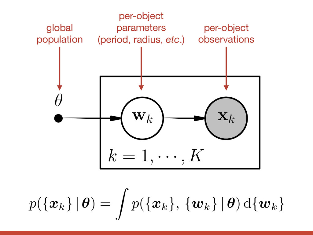
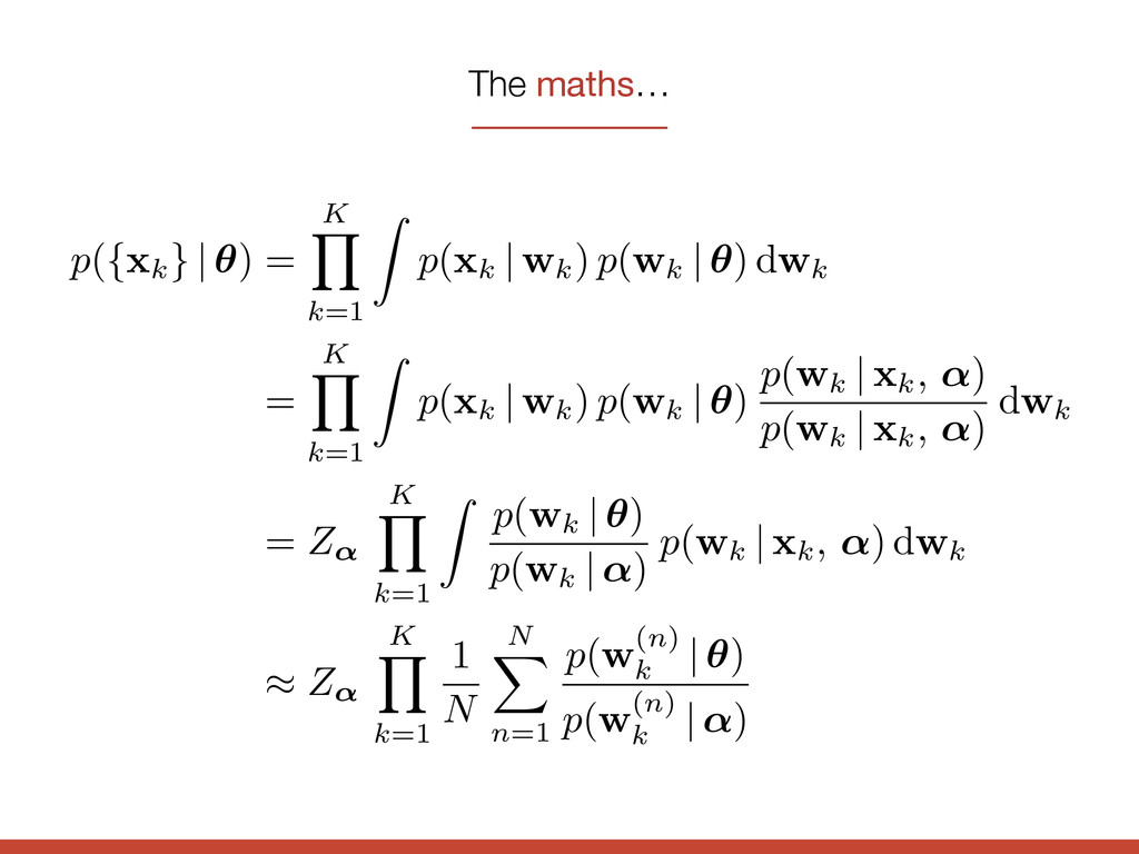
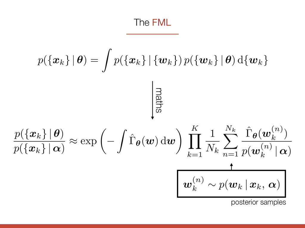
26. The maths… p({ xk } | ✓) = K Y k=1 Z p( xk | wk) p( wk | ✓) d wk = K Y k=1 Z p( xk | wk) p( wk | ✓) p( wk | xk, ↵) p( wk | xk, ↵) d wk = Z↵ K Y k=1 Z p( wk | ✓) p( wk | ↵) p( wk | xk, ↵) d wk ⇡ Z↵ K Y k=1 1 N N X n=1 p( w (n) k | ✓) p( w (n) k | ↵)
27. Hogg, Myers, & Bovy (2010) 0.0 0.2 0.4 0.6 0.8 1.0 eccentricity e 0 1 0.0 0.2 0.4 0.6 0.8 eccentricity e 0 2 0.0 0.2 0.4 0.6 0.8 1.0 eccentricity e 0 1 2 3 4 5 frequency p(e) 300 stars / ML estimates 0.0 0.2 0.4 0.6 0.8 eccentricity e 0 2 4 6 8 10 frequency p(e) 300 stars / ML estimates 3 4 5 cy p(e) 300 stars / inferred distribution 6 8 10 cy p(e) 300 stars / inferred distribution 0.0 0.2 0.4 0.6 0.8 1.0 eccentricity e 0 1 0.0 0.2 0.4 0.6 0.8 1.0 eccentricity e 0 1 2 3 4 5 frequency p(e) 300 stars / inferred distribution Fig. 2.— True, maximum-likelihood of 300 ersatz exoplanets. The top tions from which the true eccentric
28. the catalog is complete & independent the rate density function is piecewise constant the measurement uncertainties are non-negligible & known The probabilistic histogram * also ignoring false positives, etc.
29. Detection efficiency 2
30. DETECTION EFFICIENCY the dreaded
31. inverse-detection-efficiency maximum likelihood the method
32. inverse-detection-efficiency maximum likelihood the method “non-parametric” Howard et al. (2011), Dressing & Charbonneau (2013), Petigura et al. (2013), and more…
33. inverse-detection-efficiency maximum likelihood the method “non-parametric” Howard et al. (2011), Dressing & Charbonneau (2013), Petigura et al. (2013), and more… “parametric” Tabachnik & Tremaine (2002), Youdin (2011), and more…
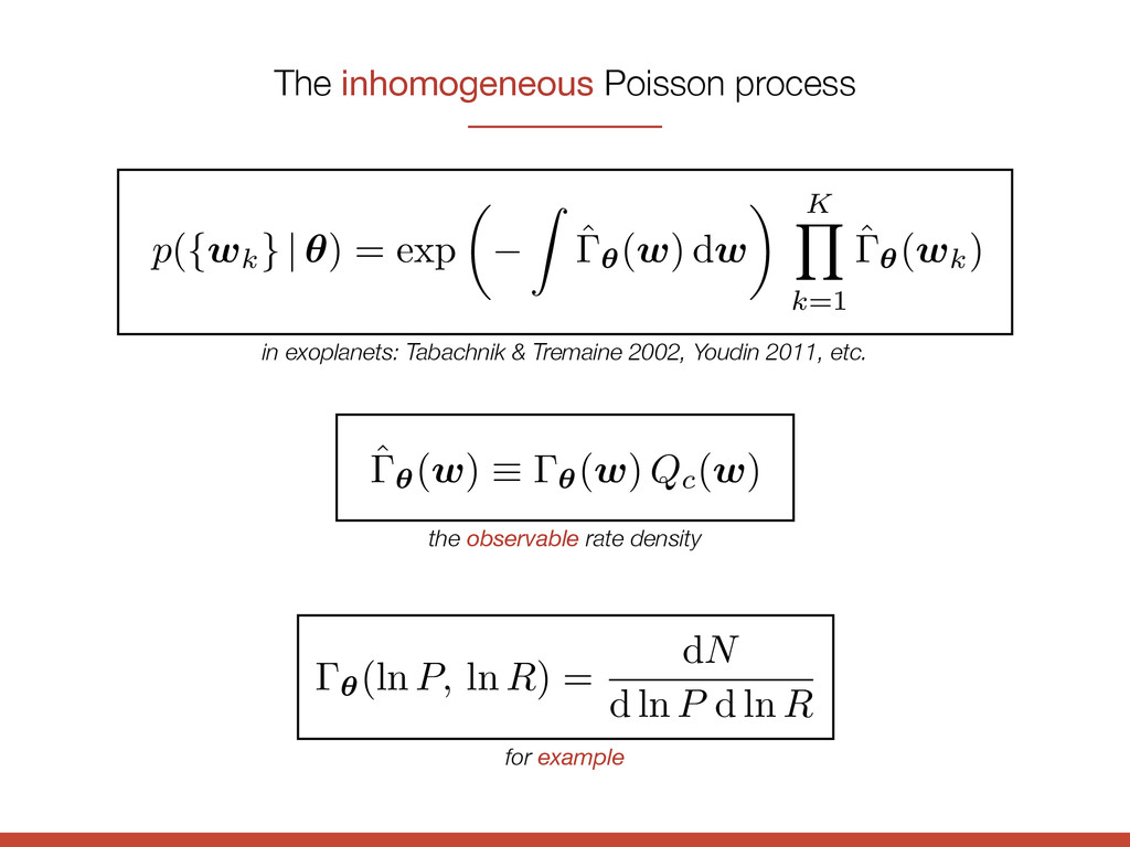
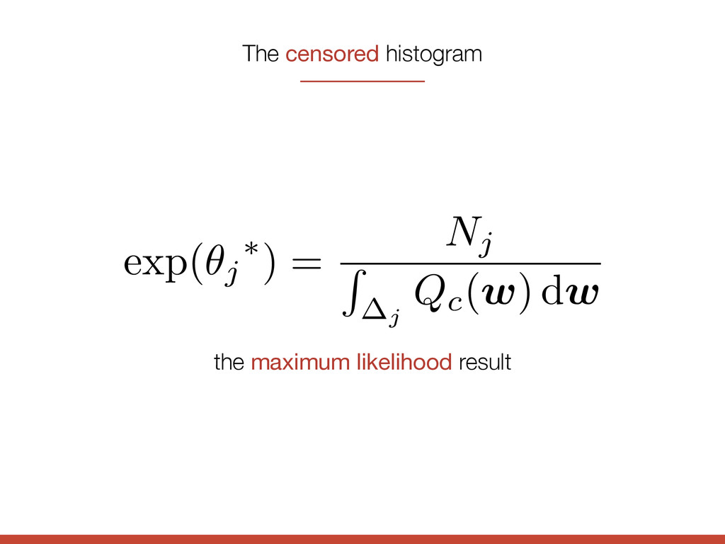
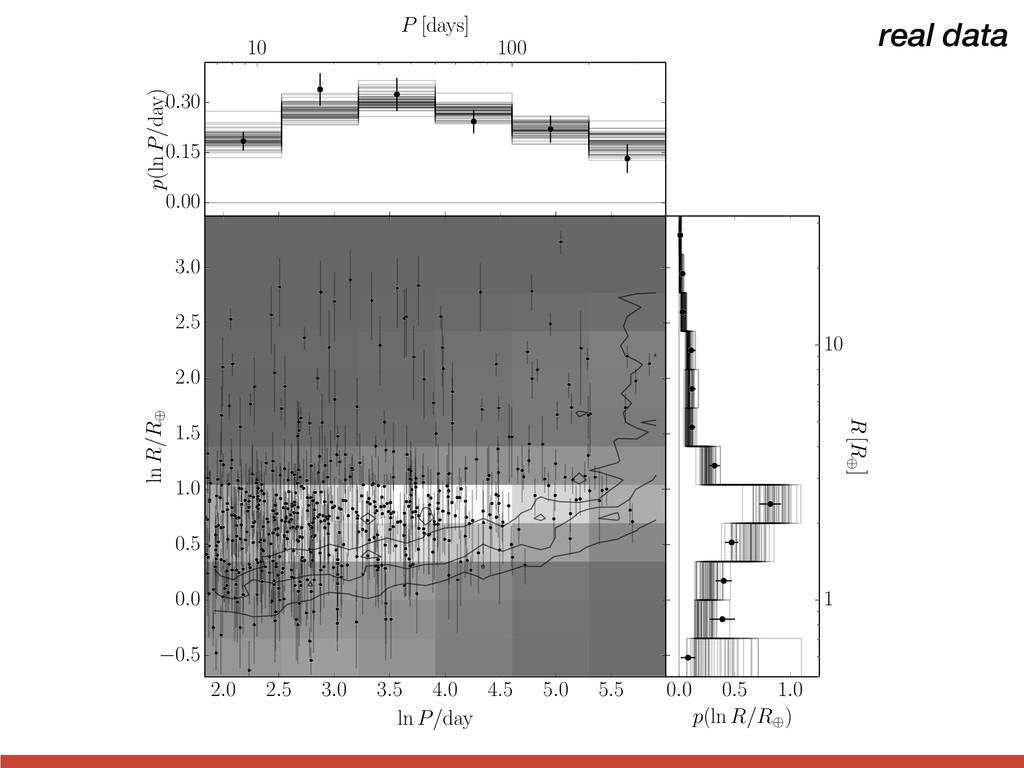
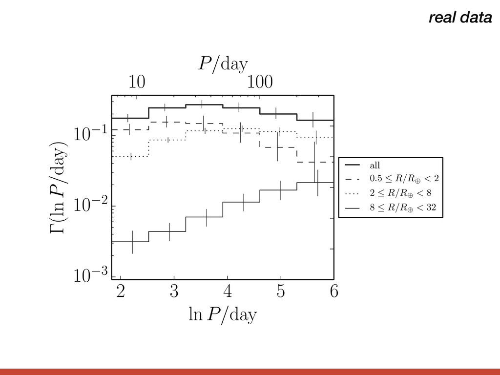
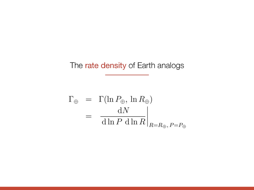
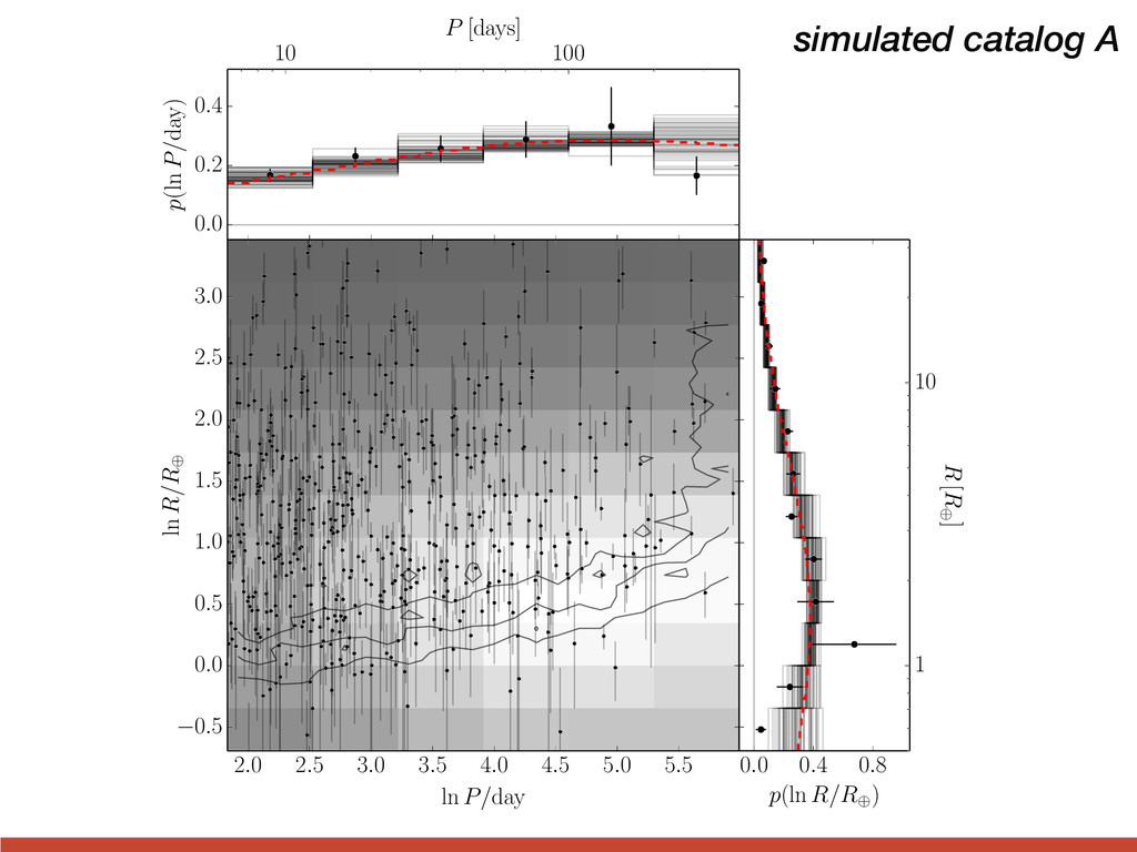
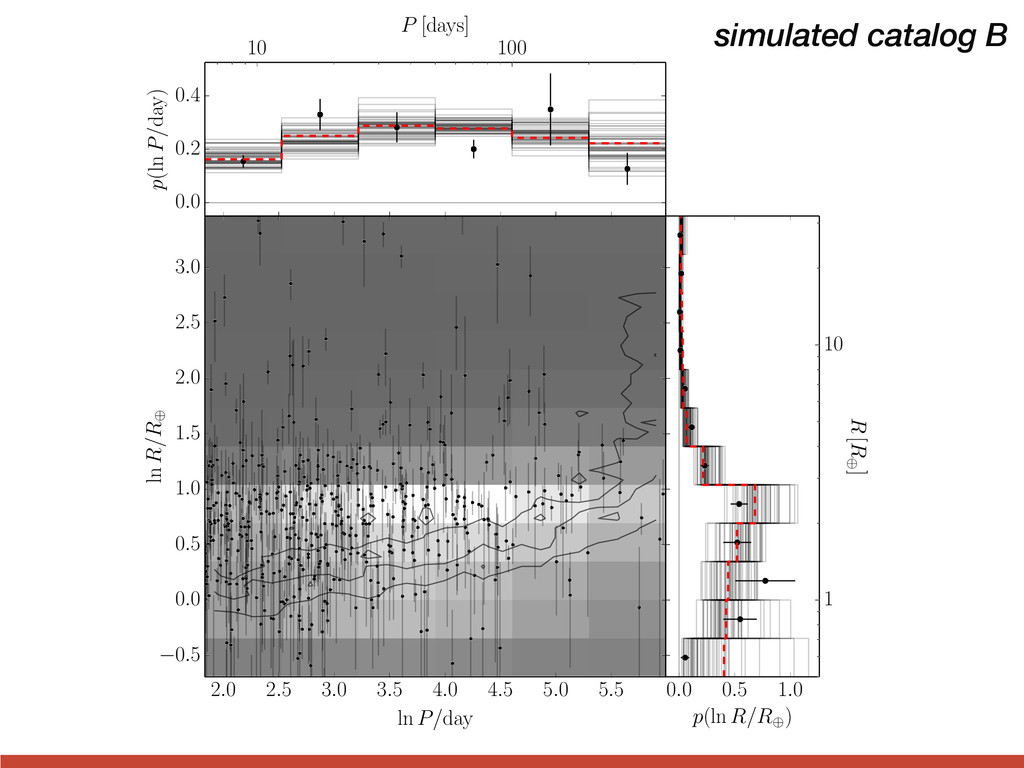
34. in exoplanets: Tabachnik & Tremaine 2002, Youdin 2011, etc. The inhomogeneous Poisson process p ( {wk } | ✓ ) = exp ✓ Z ˆ✓( w ) d w ◆ K Y k=1 ˆ✓( wk) ˆ ✓(w) ⌘ ✓(w) Qc(w) the observable rate density ✓(ln P, ln R) = dN d ln P d ln R for example
35. the true rate density model ✓( w ) = 8 > > > > < > > > > : exp( ✓1) w 2 1, exp( ✓2) w 2 2, · · · exp( ✓J ) w 2 J , 0 otherwise The censored histogram L(✓) = ln p({wk } | ✓) = J X j=1 e✓j Z j Qc(w) dw + K X k=1 J X j=1 1[wk 2 j] [ln Qc(wk) + ✓j] the Poisson log-likelihood
36. The censored histogram exp( ✓j ⇤ ) = Nj R j Qc( w ) d w the maximum likelihood result
37. the catalog is complete & independent the rate density function is piecewise constant the measurement uncertainties are negligible The censored histogram * also ignoring false positives, etc.
38. Putting it all together 3
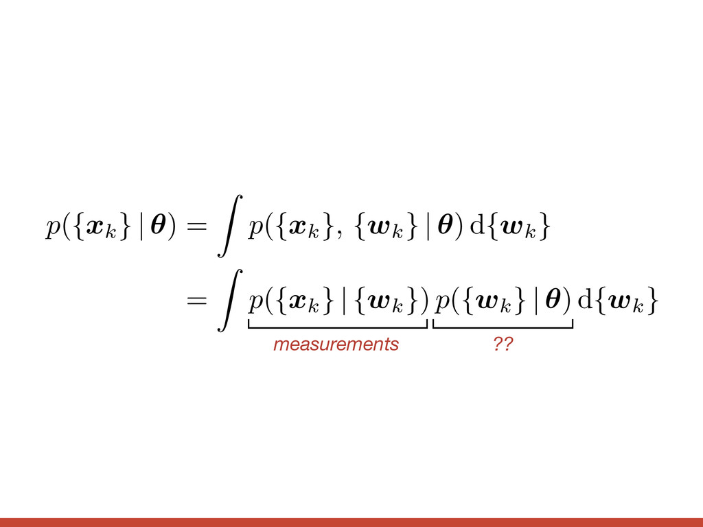
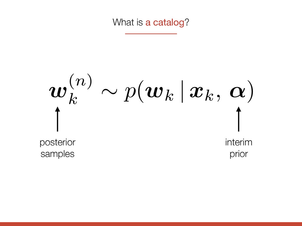
39. p ( { xk } | ✓) p ( { xk } | ↵) ⇡ exp ✓ Z ˆ✓(w) dw ◆ K Y k=1 1 Nk Nk X n=1 ˆ✓(w (n) k ) p (w (n) k | ↵) p({ xk } | ✓ ) = Z p({ xk } | { wk }) p({ wk } | ✓ ) d{ wk } The FML maths w (n) k ⇠ p( wk | xk, ↵ ) posterior samples
40. the catalog is complete & independent the rate density function is anything the measurement uncertainties are non-negligible & known The probabilistic, censored “histogram” * also ignoring false positives, etc.
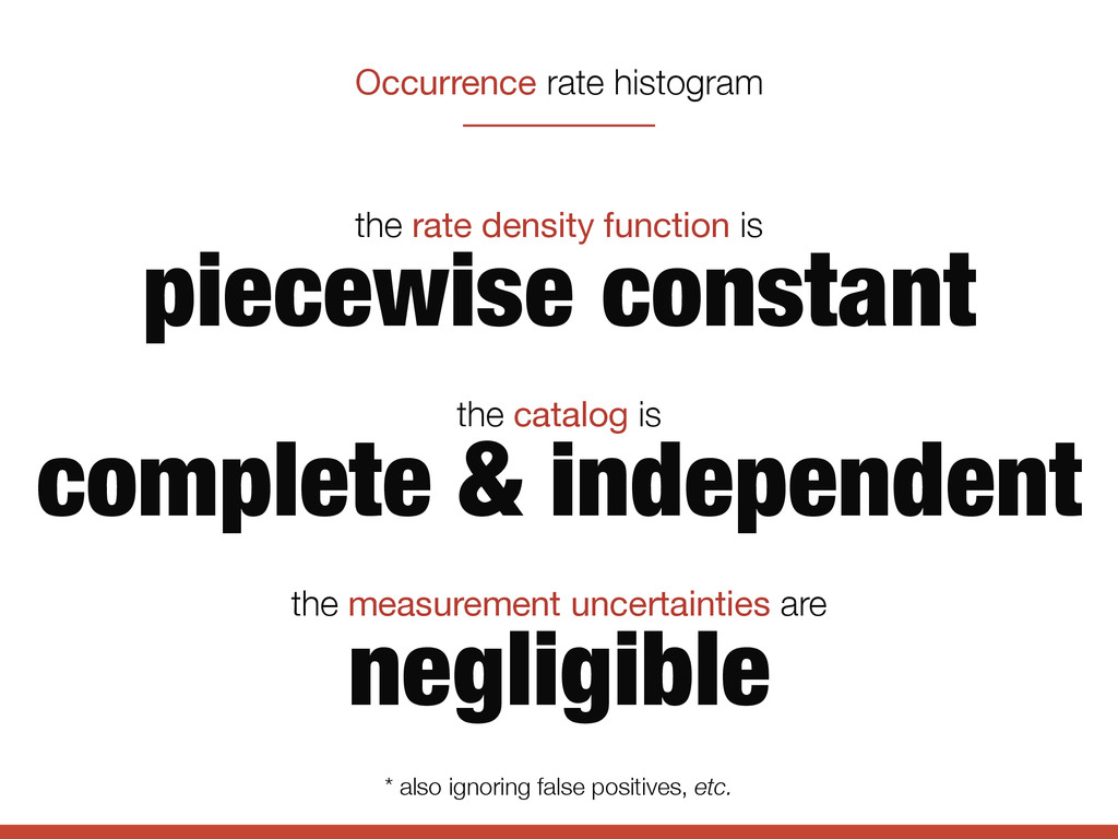
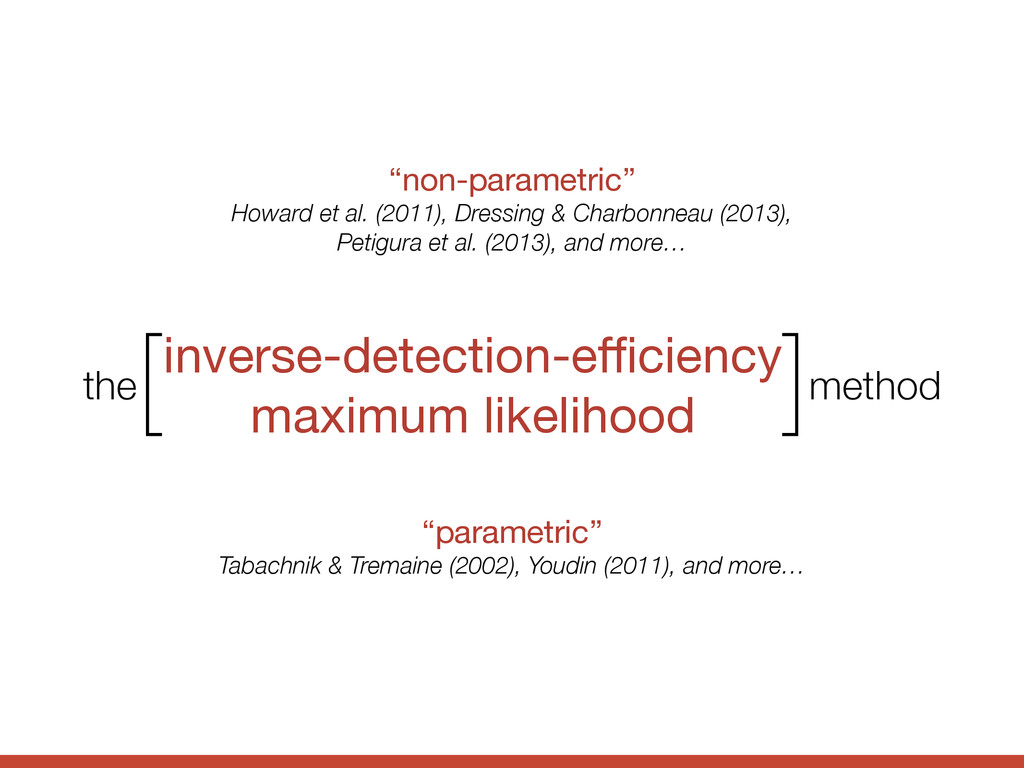
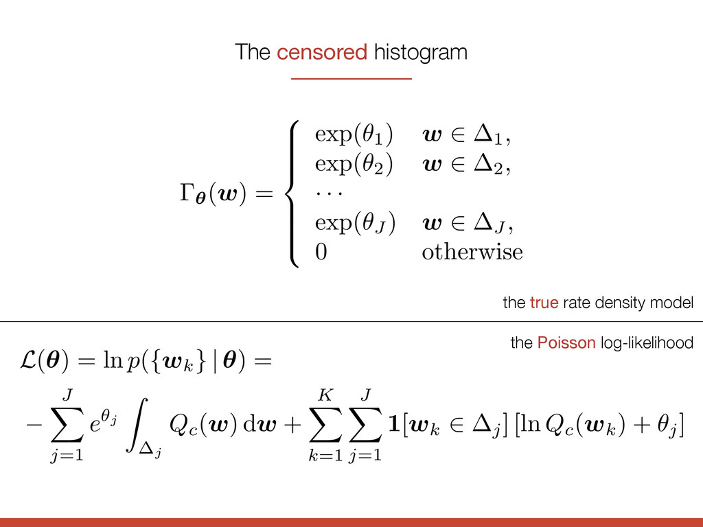
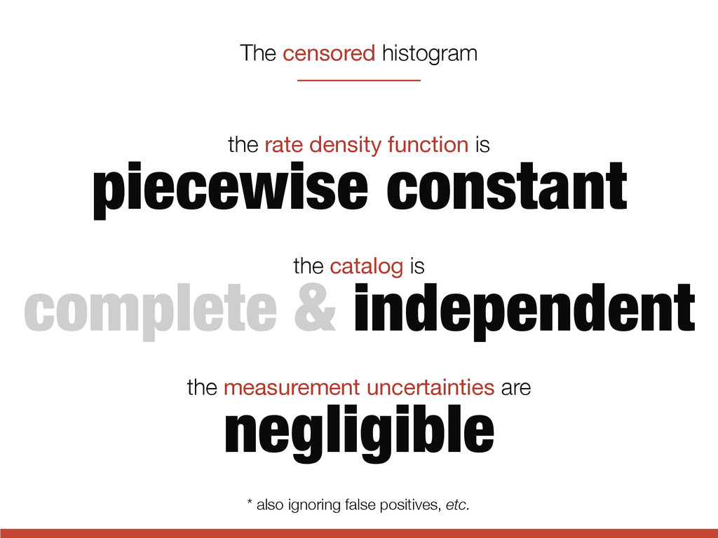
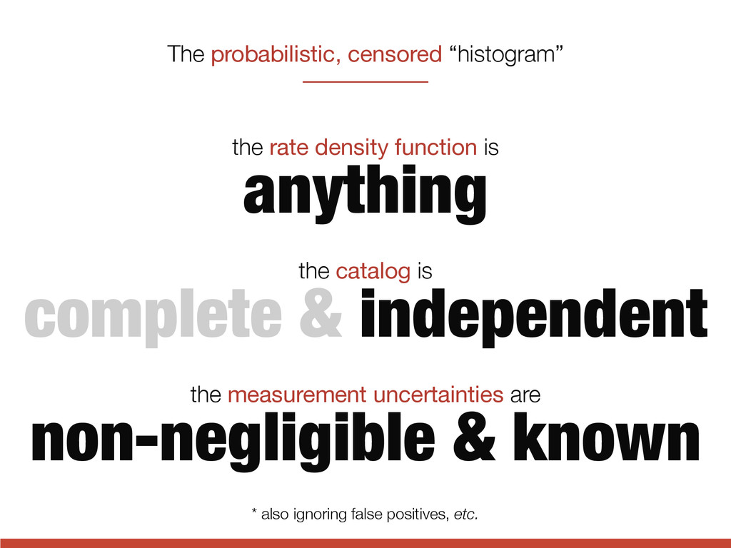
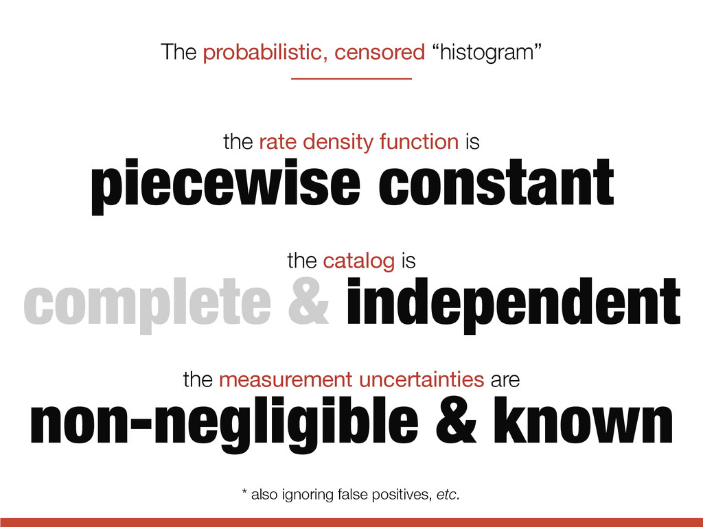
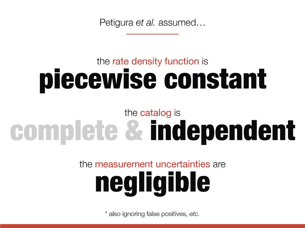
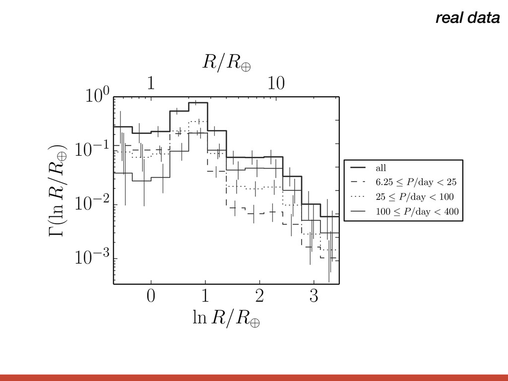
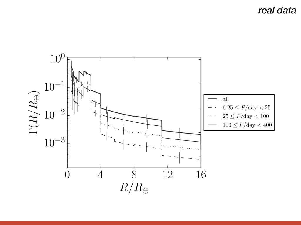
41. the catalog is complete & independent the rate density function is piecewise constant the measurement uncertainties are non-negligible & known The probabilistic, censored “histogram” * also ignoring false positives, etc.
42. The data 4
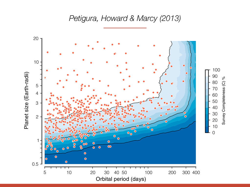
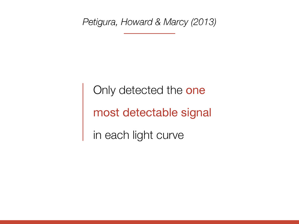
43. color-coded as a function of P and RP . The survey completeness for small planets is a complicated function of P and RP . It decreases with increasing P and decreasing both completeness factors). stars have a planet with pe between 1 and 2 R⊕ . 5 10 20 30 40 50 100 200 300 400 Orbital period (days) 0.5 1 2 3 4 5 10 20 Planet size (Earth-radii) 0 10 20 30 40 50 60 70 80 90 100 Survey Completeness (C) % Fig. 1. on a lo detected like star color sca injection photom complet missed rence. T orbital P graph). orbital favors d Petigura, Howard & Marcy (2013)
44. Only detected the one most detectable signal in each light curve Petigura, Howard & Marcy (2013)
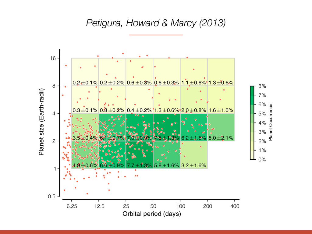
45. 6.25 12.5 25 50 100 200 400 Orbital period (days) 0.5 1 2 4 8 16 Planet size (Earth-radii) 4.9 0.6% 3.5 0.4% 0.3 0.1% 0.2 0.1% 6.6 0.9% 6.1 0.7% 0.8 0.2% 0.2 0.2% 7.7 1.3% 7.0 0.9% 0.4 0.2% 0.6 0.3% 5.8 1.6% 7.5 1.3% 1.3 0.6% 0.6 0.3% 3.2 1.6% 6.2 1.5% 2.0 0.8% 1.1 0.6% 5.0 2.1% 1.6 1.0% 1.3 0.6% 0% 1% 2% 3% 4% 5% 6% 7% 8% Planet Occurrence Fig. 2. Plan orbital perio d and RP = 0: are shown as in orbital pe in a cell is where the su each cell. He planets (for of the orbita completenes Best42k sam planet occur occurrence w where the c the small pl rence is cons entire range ports mild e RP = 1 − 2 R⊕ Petigura, Howard & Marcy (2013)
46. the catalog is complete & independent the rate density function is piecewise constant the measurement uncertainties are negligible Petigura et al. assumed… * also ignoring false positives, etc.
47. 2.0 2.5 3.0 3.5 4.0 4.5 5.0 5.5 ln P/day 0.5 0.0 0.5 1.0 1.5 2.0 2.5 3.0 ln R/R 0.00 0.15 0.30 p(ln P/day) 0.0 0.5 1.0 p(ln R/R ) 10 100 P [days] 1 10 R [R ] real data
48. 2 3 4 5 6 ln P/day 10 3 10 2 10 1 (ln P/day) all 0.5  R/R < 2 2  R/R < 8 8  R/R < 32 10 100 P/day real data
49. 0 1 2 3 ln R/R 10 3 10 2 10 1 100 (ln R/R ) all 6.25  P/day < 25 25  P/day < 100 100  P/day < 400 1 10 R/R real data
50. 0 4 8 12 16 R/R 10 3 10 2 10 1 100 (R/R ) all 6.25  P/day < 25 25  P/day < 100 100  P/day < 400 real data
51. CARE? why should I
52. 2.0 2.5 3.0 3.5 4.0 4.5 5.0 5.5 ln P/day 0.5 0.0 0.5 1.0 1.5 2.0 2.5 3.0 ln R/R 0.0 0.2 0.4 p(ln P/day) 0.0 0.4 0.8 p(ln R/R ) 10 100 P [days] 1 10 R [R ] simulated catalog A
53. 2.0 2.5 3.0 3.5 4.0 4.5 5.0 5.5 ln P/day 0.5 0.0 0.5 1.0 1.5 2.0 2.5 3.0 ln R/R 0.0 0.2 0.4 p(ln P/day) 0.0 0.5 1.0 p(ln R/R ) 10 100 P [days] 1 10 R [R ] simulated catalog B
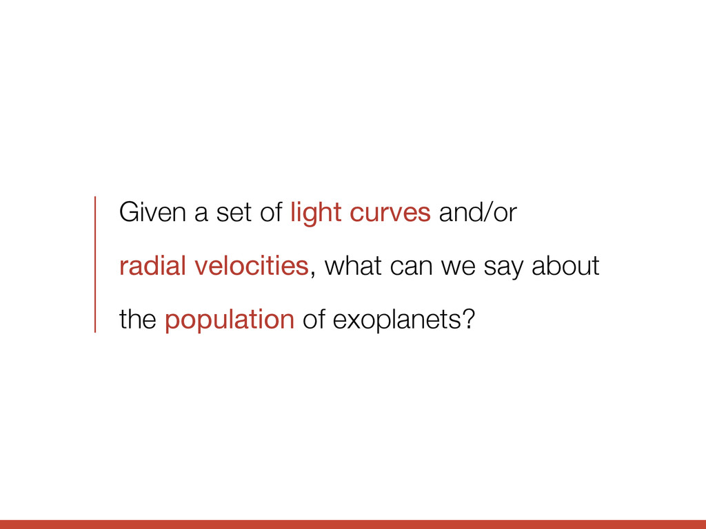
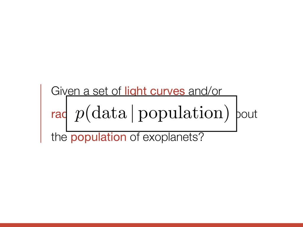
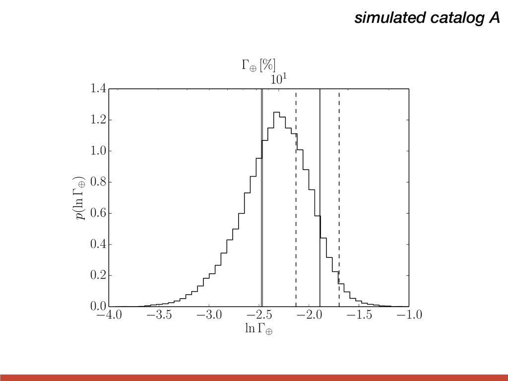
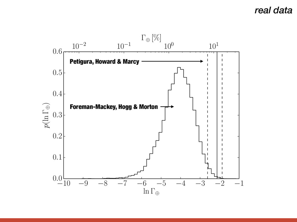
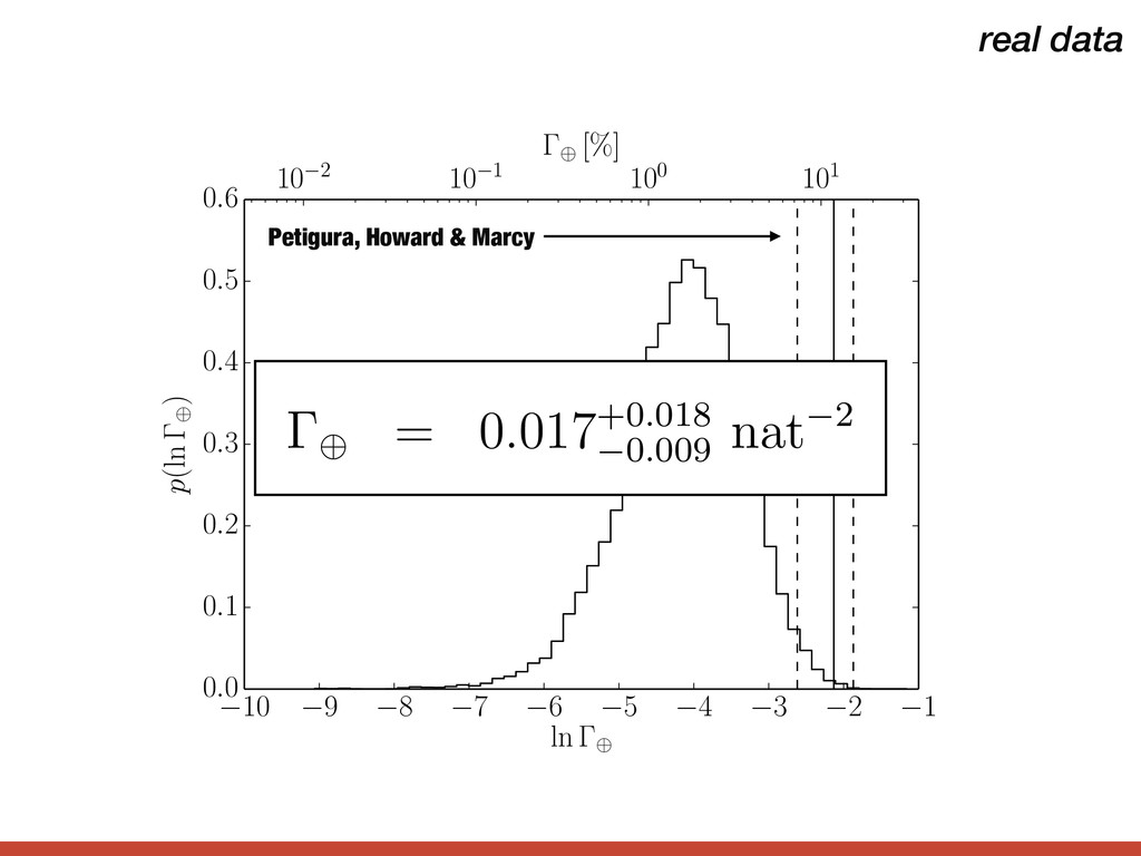
54. The rate density of Earth analogs ing distribution. 6. Extrapolation to Earth well as inferring the occurrence distribution of exoplanets, this dataset constrain the rate density of Earth analogs. Explicitly, we constrain the nsity of exoplanets orbiting “Sun-like” stars11, evaluated at the location = (ln P , ln R ) = dN d ln P d ln R R=R , P=P . is the rate density of exoplanets around a Sun-like star (expected per star per natural logarithm of period per natural logarithm of radius eriod and radius of Earth. Equation (23), we define “Earth analog” in terms of measurable quantit
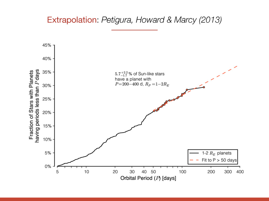
55. action of stars having nearly Earth-size planets ð1 − 2 R⊕Þ with any orbital period up to a maximum period, P, on the horiz rly Earth size ð1 − 2 R⊕Þ are included. This cumulative distribution reaches 20.2% at P = 50 d, meaning 20.4% of Sun-like stars Extrapolation: Petigura, Howard & Marcy (2013)
56. Extrapolation: Foreman-Mackey, Hogg & Morton (submitted) Gaussian Process use a the rate function should be “smooth”
57. 2.0 2.5 3.0 3.5 4.0 4.5 5.0 5.5 ln P/day 0.5 0.0 0.5 1.0 1.5 2.0 2.5 3.0 ln R/R 0.0 0.2 0.4 p(ln P/day) 0.0 0.4 0.8 p(ln R/R ) 10 100 P [days] 1 10 R [R ] simulated catalog A
58. 4.0 3.5 3.0 2.5 2.0 1.5 1.0 ln 0.0 0.2 0.4 0.6 0.8 1.0 1.2 1.4 p(ln ) 101 [%] simulated catalog A
59. 2.0 2.5 3.0 3.5 4.0 4.5 5.0 5.5 ln P/day 0.5 0.0 0.5 1.0 1.5 2.0 2.5 3.0 ln R/R 0.0 0.2 0.4 p(ln P/day) 0.0 0.5 1.0 p(ln R/R ) 10 100 P [days] 1 10 R [R ] simulated catalog B
60. 6 5 4 3 2 1 0 ln 0.0 0.1 0.2 0.3 0.4 0.5 0.6 p(ln ) 100 101 102 [%] simulated catalog B
61. 2.0 2.5 3.0 3.5 4.0 4.5 5.0 5.5 ln P/day 0.5 0.0 0.5 1.0 1.5 2.0 2.5 3.0 ln R/R 0.00 0.15 0.30 p(ln P/day) 0.0 0.5 1.0 p(ln R/R ) 10 100 P [days] 1 10 R [R ] real data
62. 10 9 8 7 6 5 4 3 2 1 ln 0.0 0.1 0.2 0.3 0.4 0.5 0.6 p(ln ) 10 2 10 1 100 101 [%] real data Foreman-Mackey, Hogg & Morton Petigura, Howard & Marcy
63. 10 9 8 7 6 5 4 3 2 1 ln 0.0 0.1 0.2 0.3 0.4 0.5 0.6 p(ln ) 10 2 10 1 100 101 [%] real data Foreman-Mackey, Hogg & Morton Petigura, Howard & Marcy on the rate density of Earth analogs (as defined h our result has large fractional uncertainty—with This is shown in Figure 9 where we compare the m for to the published value and uncertainty. Qu y of Earth analogs is = 0.017+0.018 0.009 nat 2 dicates that this quantity is a rate density, per natur mic radius. Converted to these units, Petigura et a the same quantity (indicated as the vertical lines in hat Petigura’s extrapolation model predicts but, for ferred rate density over their choice of “Earth-like”
64. Conclusions & Summary. 4
65. the catalog is complete & independent the rate density function is anything the measurement uncertainties are non-negligible & known * also ignoring false positives, etc.