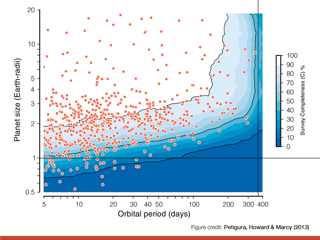
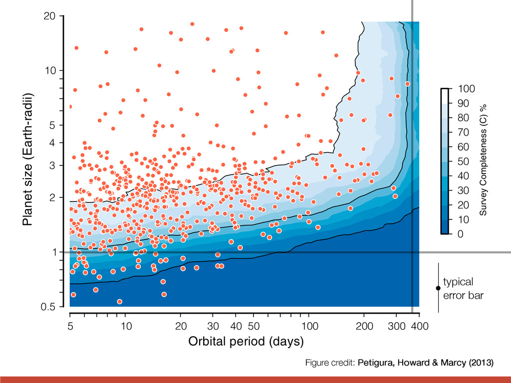
Orbital period (days) 0.5 1 2 3 4 5 10 20 Planet size (Earth-radii) 0 10 20 30 40 50 60 70 80 90 100 Survey Completeness (C) % F o d li c in p c m r o g o f Figure credit: Petigura, Howard & Marcy (2013)
Orbital period (days) 0.5 1 2 3 4 5 10 20 Planet size (Earth-radii) 0 10 20 30 40 50 60 70 80 90 100 Survey Completeness (C) % F o d li c in p c m r o g o f Figure credit: Petigura, Howard & Marcy (2013)
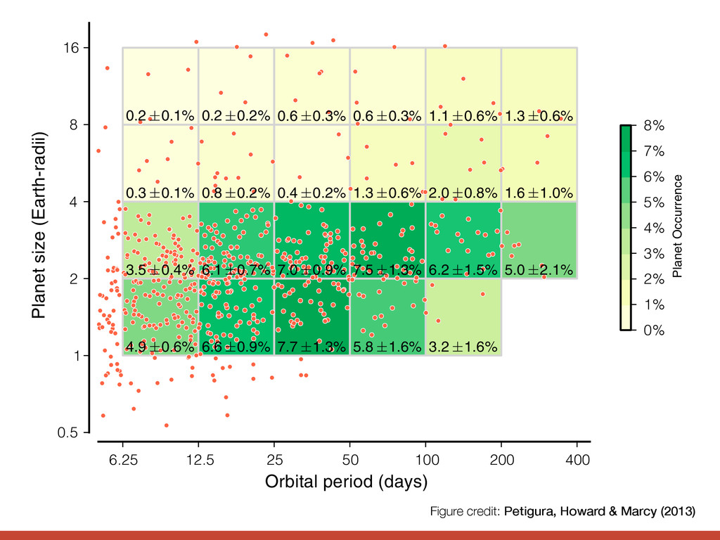
0.5 1 2 4 8 16 Planet size (Earth-radii) 4.9 0.6% 3.5 0.4% 0.3 0.1% 0.2 0.1% 6.6 0.9% 6.1 0.7% 0.8 0.2% 0.2 0.2% 7.7 1.3% 7.0 0.9% 0.4 0.2% 0.6 0.3% 5.8 1.6% 7.5 1.3% 1.3 0.6% 0.6 0.3% 3.2 1.6% 6.2 1.5% 2.0 0.8% 1.1 0.6% 5.0 2.1% 1.6 1.0% 1.3 0.6% 0% 1% 2% 3% 4% 5% 6% 7% 8% Planet Occurrence Fi o d a in in w e p o co B p o w th re e p R Figure credit: Petigura, Howard & Marcy (2013)
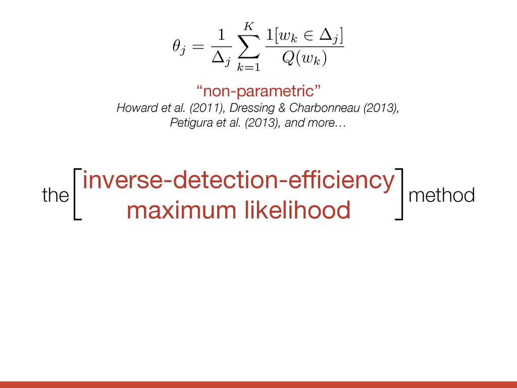
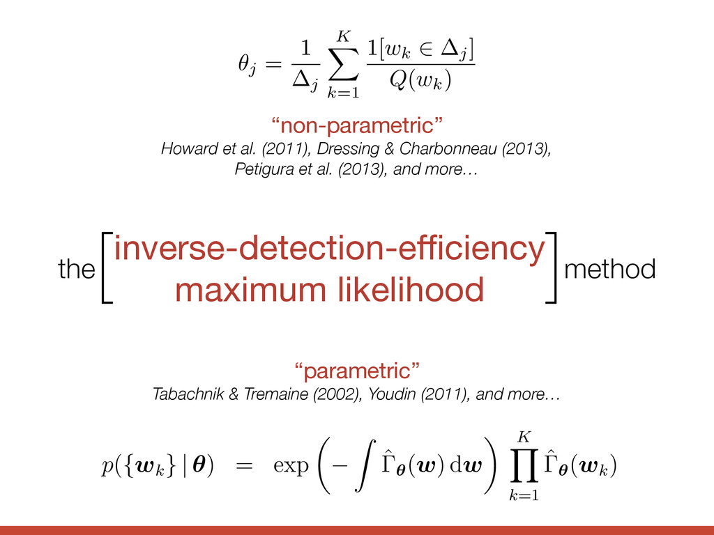
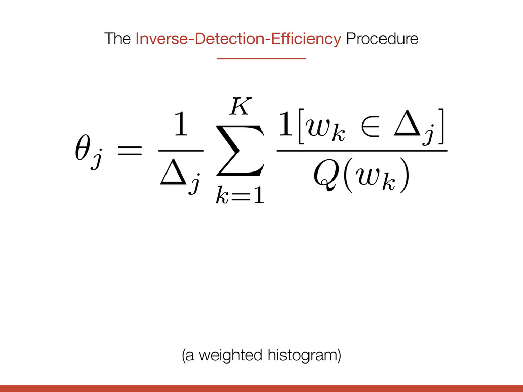
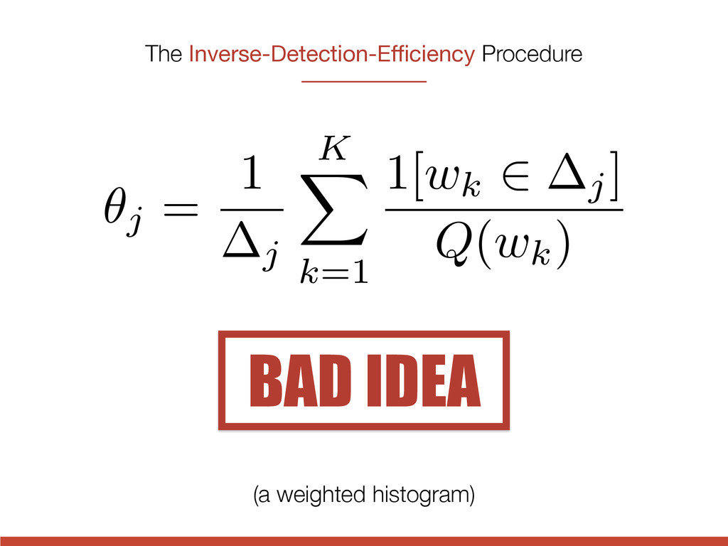
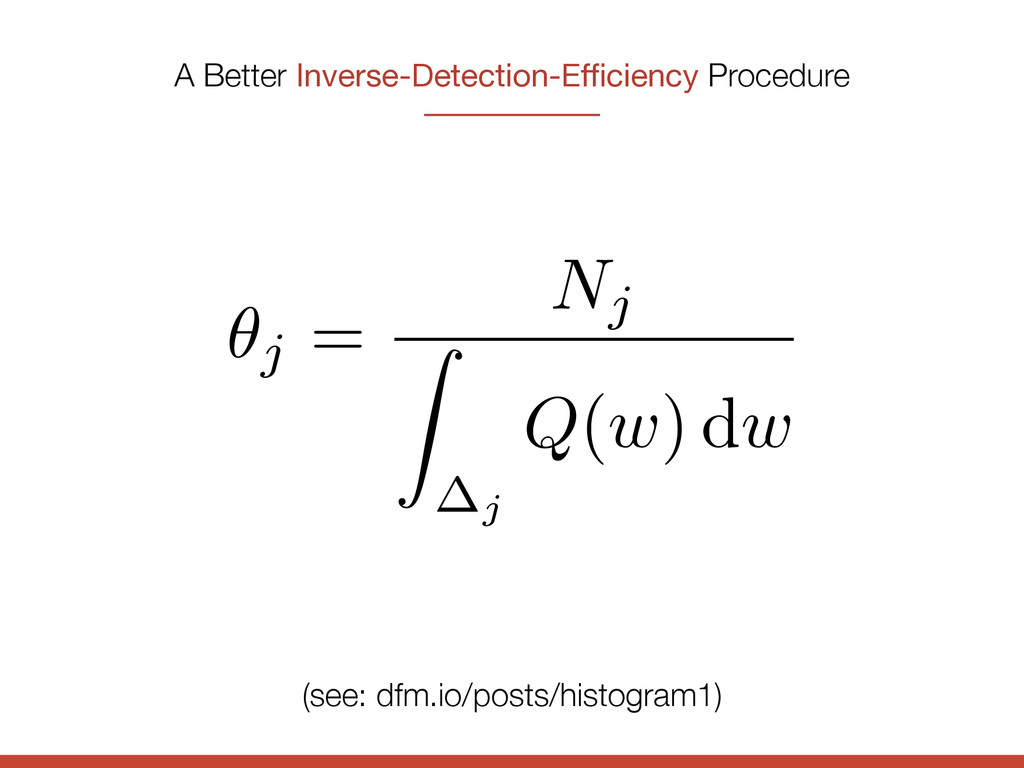
Dressing & Charbonneau (2013), Petigura et al. (2013), and more… ✓j = 1 j K X k=1 1[wk 2 j] Q(wk) “parametric” Tabachnik & Tremaine (2002), Youdin (2011), and more… – 6 – e 2002; Youdin 2011 for some of the examples from the exoplanet litera p({ wk } | ✓ ) = exp ✓ Z ˆ ✓ ( w ) d w ◆ K Y k=1 ˆ ✓ ( wk ) .
Orbital period (days) 0.5 1 2 3 4 5 10 20 Planet size (Earth-radii) 0 10 20 30 40 50 60 70 80 90 100 Survey Completeness (C) % F o d li c in p c m r o g o f Figure credit: Petigura, Howard & Marcy (2013) typical error bar
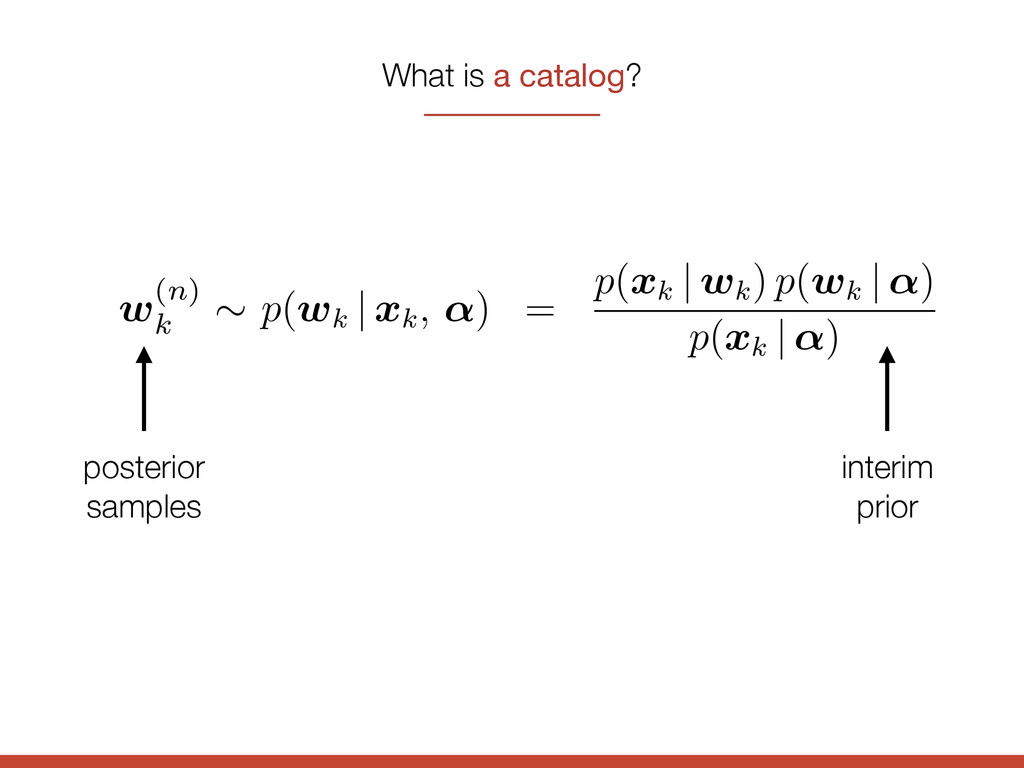
k ⇠ p( wk | xk, ↵ ) – 8 – d, we will reuse the hard work that went into building the c each entry in a catalog is a representation of the posterior p( wk | xk , ↵ ) = p( xk | wk ) p( wk | ↵ ) p( xk | ↵ ) ameters wk conditioned on the observations of that objec minder that the catalog was produced under a specific c tive”— interim prior p( wk | ↵ ). This prior was chosen by th s di↵erent from the likelihood p( wk | ✓ ) from Equation (2). we can use these posterior measurements to simplify Equ n many common cases, be evaluated e ciently. To find thi
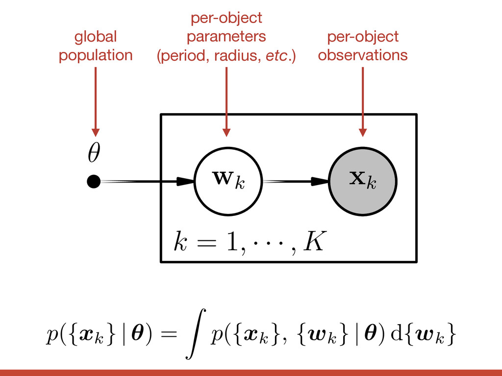
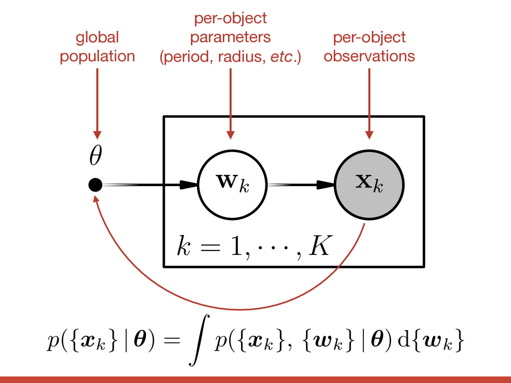
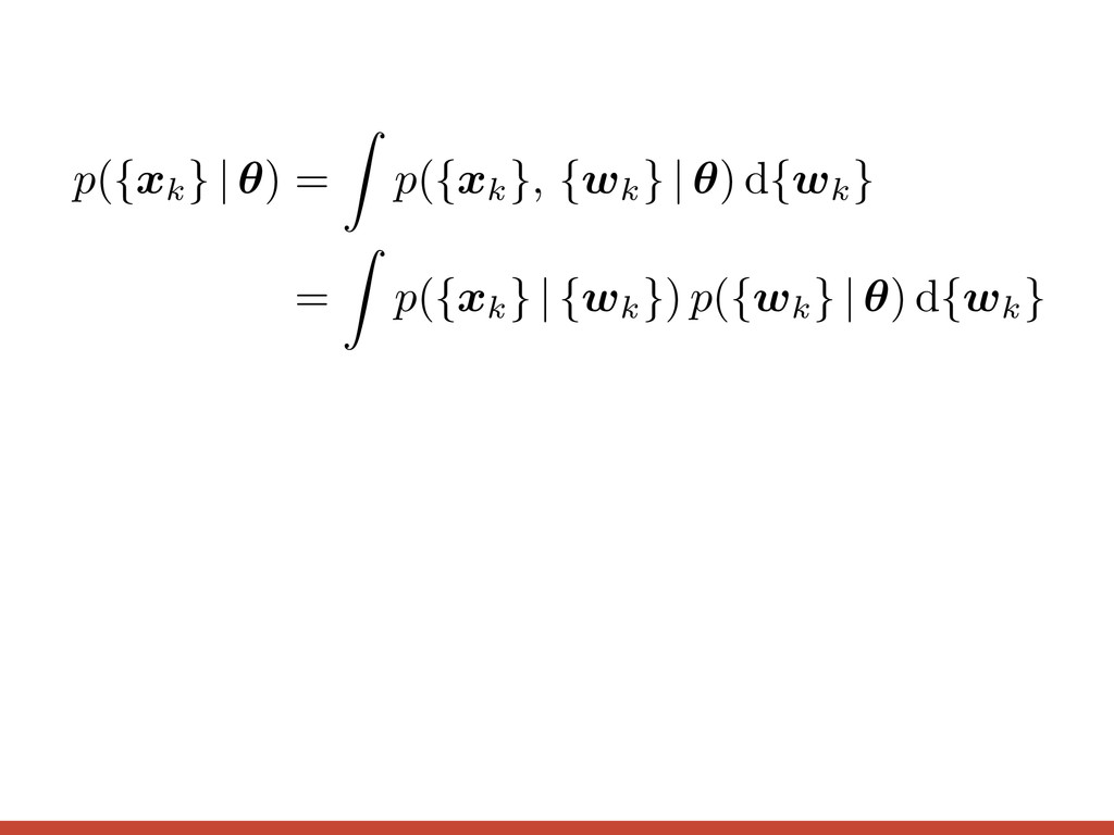
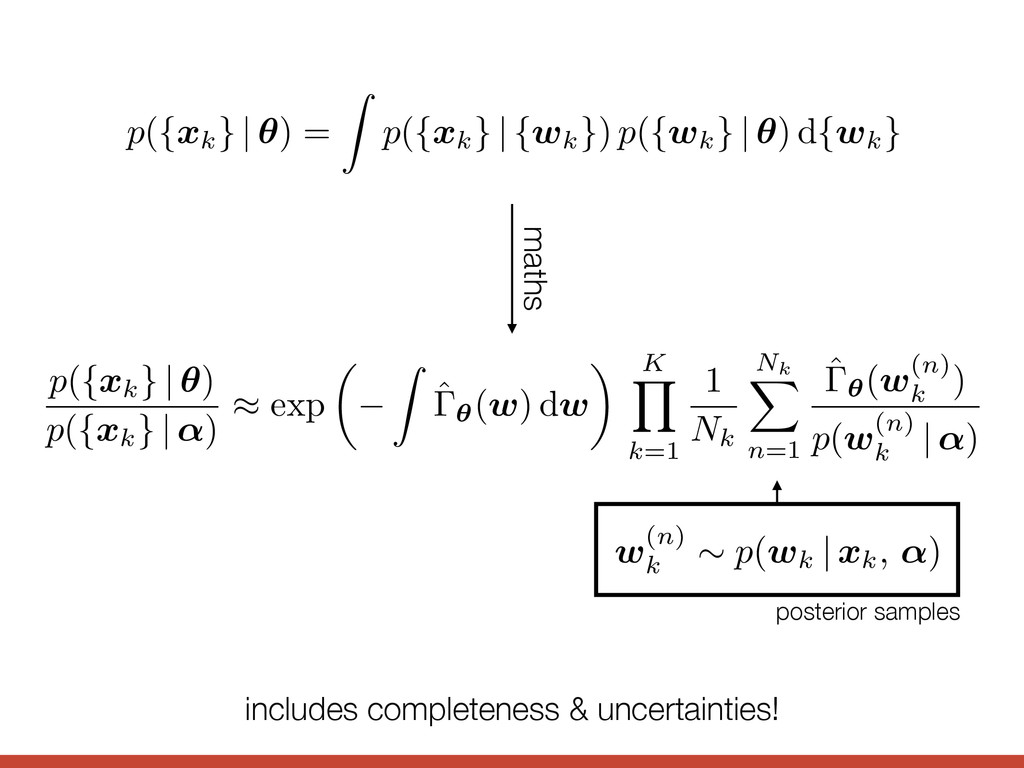
xk } | ↵) ⇡ exp ✓ Z ˆ✓(w) dw ◆ K Y k=1 1 Nk Nk X n=1 ˆ✓(w (n) k ) p (w (n) k | ↵) p({ xk } | ✓ ) = Z p({ xk } | { wk }) p({ wk } | ✓ ) d{ wk } maths w (n) k ⇠ p( wk | xk, ↵ ) posterior samples includes completeness & uncertainties!
pixels given population expected # of observable exoplanets p ( { xk } | ✓) p ( { xk } | ↵) ⇡ exp ✓ Z ˆ✓(w) dw ◆ K Y k=1 1 Nk Nk X n=1 ˆ✓(w (n) k ) p (w (n) k | ↵) sum over posterior samples product over objects The "Money Equation™"
pixels given population expected # of observable exoplanets p ( { xk } | ✓) p ( { xk } | ↵) ⇡ exp ✓ Z ˆ✓(w) dw ◆ K Y k=1 1 Nk Nk X n=1 ˆ✓(w (n) k ) p (w (n) k | ↵) sum over posterior samples product over objects The "Money Equation™"
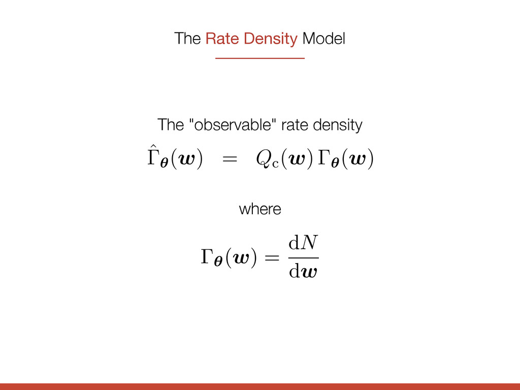
is that ˆ ✓ is the rate density of exo observe taking into account the geometric transit probabil cies. In practice, we can model the observable rate density ˆ ✓ ( w ) = Qc ( w ) ✓ ( w ) he detection e ciency (including transit probability) at w ant to infer: the True occurrence rate density. We haven’t al form for ✓ ( w ) and all of this derivation is equally appli ensity as, for example, a broken power law or a histogram d rate density ˆ is a quantitative description of the rate n the Petigura et al. (2013b) catalog; it is not a description ✓(w) = dN dw The "observable" rate density where
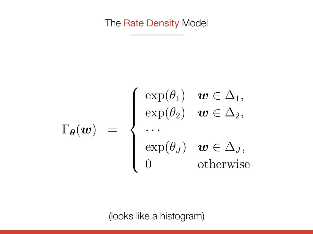
functional form for the ameters along with the parameters of the rate density. all the results in this Article, we’ll model the rate dens nction ✓ ( w ) = 8 > > > > > < > > > > > : exp(✓1 ) w 2 1 , exp(✓2 ) w 2 2 , · · · exp(✓J ) w 2 J , 0 otherwise eters ✓j are the log step heights and the bins j are fixed (looks like a histogram)
0.5 1 2 4 8 16 Planet size (Earth-radii) 4.9 0.6% 3.5 0.4% 0.3 0.1% 0.2 0.1% 6.6 0.9% 6.1 0.7% 0.8 0.2% 0.2 0.2% 7.7 1.3% 7.0 0.9% 0.4 0.2% 0.6 0.3% 5.8 1.6% 7.5 1.3% 1.3 0.6% 0.6 0.3% 3.2 1.6% 6.2 1.5% 2.0 0.8% 1.1 0.6% 5.0 2.1% 1.6 1.0% 1.3 0.6% 0% 1% 2% 3% 4% 5% 6% 7% 8% Planet Occurrence Fi o d a in in w e p o co B p o w th re e p R Figure credit: Petigura, Howard & Marcy (2013)
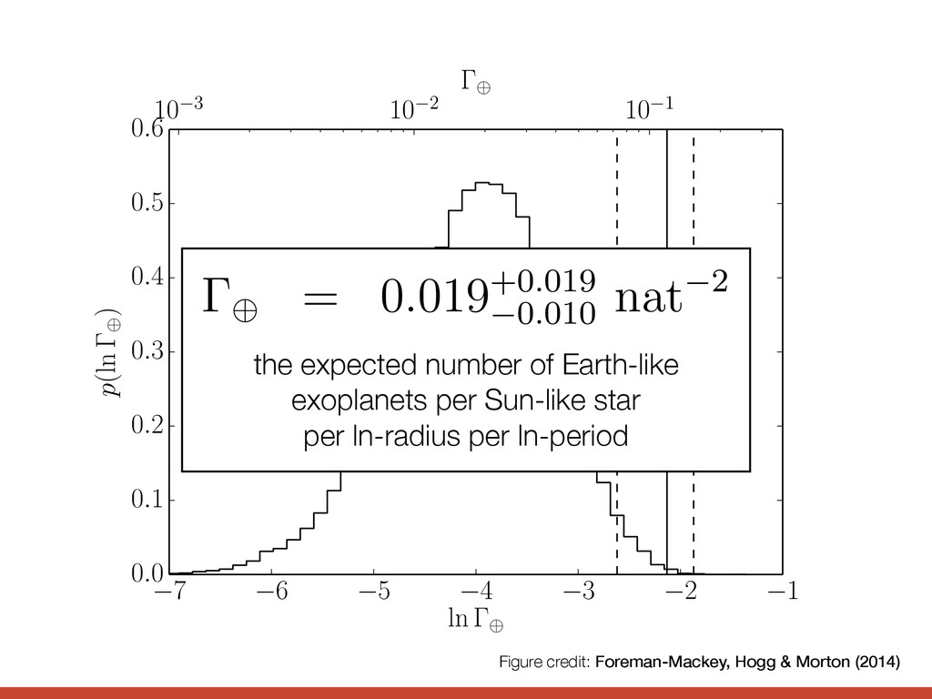
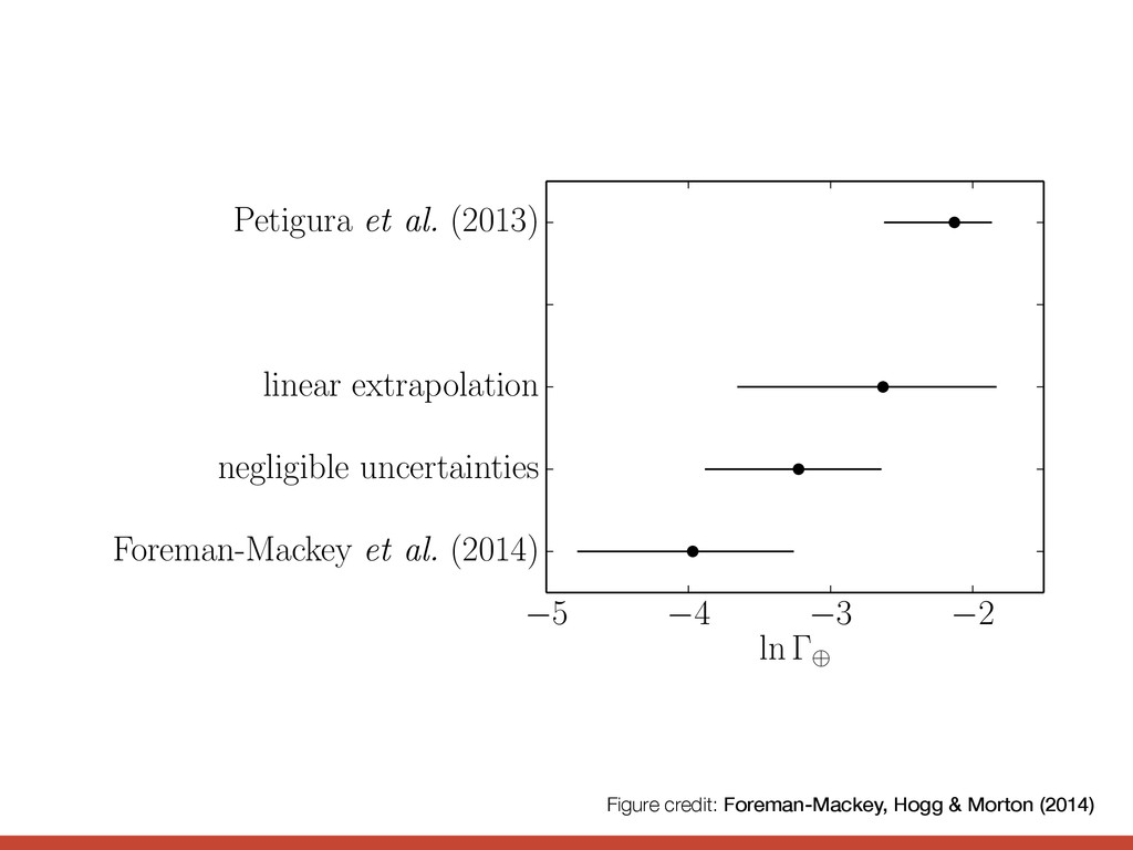
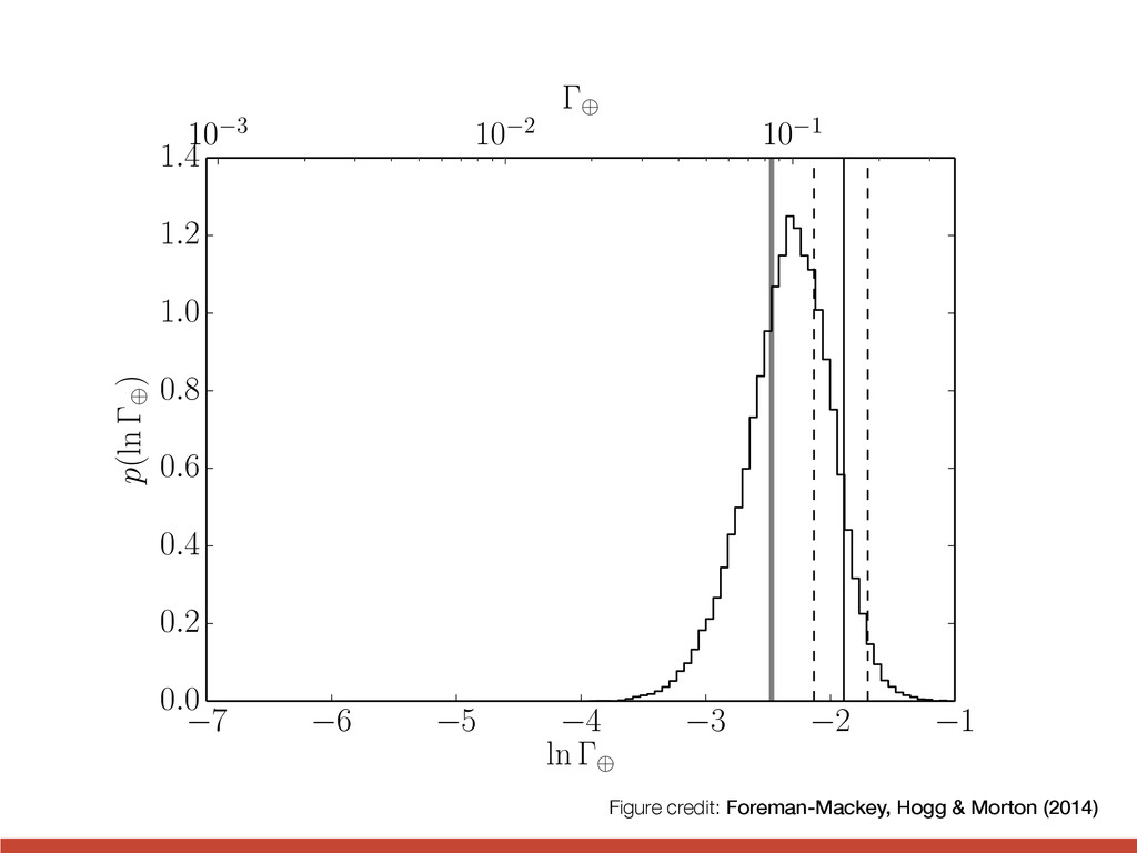
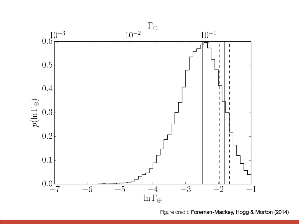
4 3 2 1 ln 0.0 0.1 0.2 0.3 0.4 0.5 0.6 p(ln ) 10 3 10 2 10 1 our result has large fractional uncertainty—w his is shown in Figure 9 where we compare the to the published value and uncertainty. Earth analogs is = 0.019+0.019 0.010 nat 2 ates that this quantity is a rate density, per na radius. Converted to these units, Petigura e same quantity (indicated as the vertical lines the expected number of Earth-like exoplanets per Sun-like star per ln-radius per ln-period
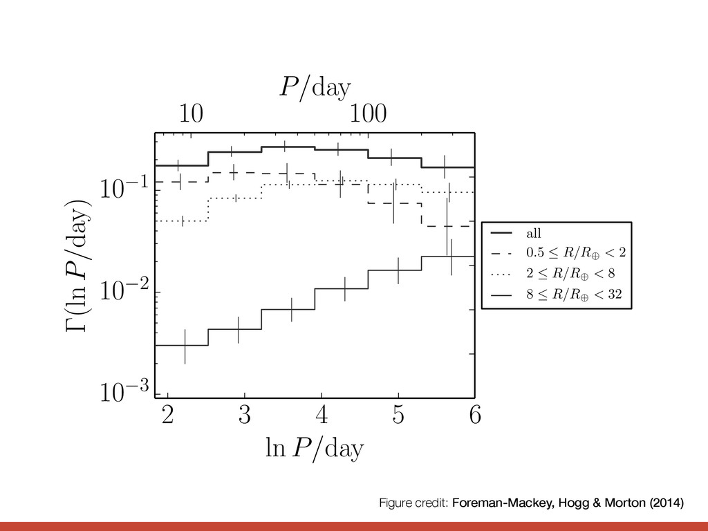
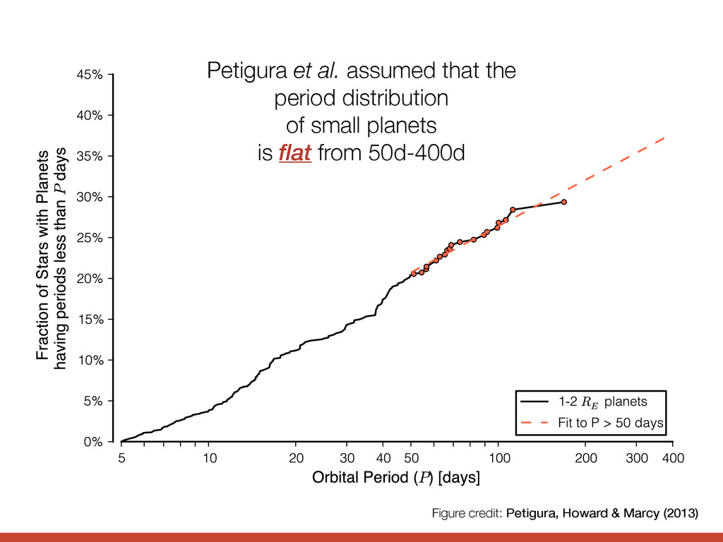
nearly Earth-size planets ð1 − 2 R⊕Þ with any orbital period up to a maximum period, P, on the h size ð1 − 2 R⊕Þ are included. This cumulative distribution reaches 20.2% at P = 50 d, meaning 20.4% of Sun-like Petigura et al. assumed that the period distribution of small planets is flat from 50d-400d
0.5 1 2 4 8 16 Planet size (Earth-radii) 4.9 0.6% 3.5 0.4% 0.3 0.1% 0.2 0.1% 6.6 0.9% 6.1 0.7% 0.8 0.2% 0.2 0.2% 7.7 1.3% 7.0 0.9% 0.4 0.2% 0.6 0.3% 5.8 1.6% 7.5 1.3% 1.3 0.6% 0.6 0.3% 3.2 1.6% 6.2 1.5% 2.0 0.8% 1.1 0.6% 5.0 2.1% 1.6 1.0% 1.3 0.6% 0% 1% 2% 3% 4% 5% 6% 7% 8% Planet Occurrence Fi o d a in in w e p o co B p o w th re e p R Figure credit: Petigura, Howard & Marcy (2013)
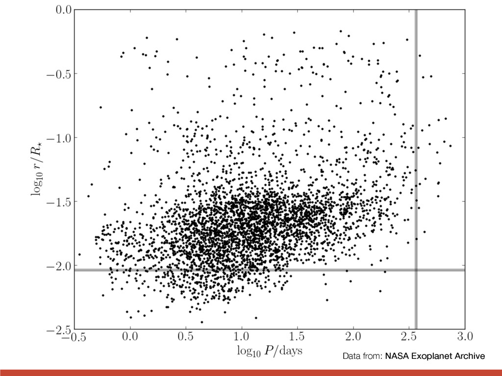
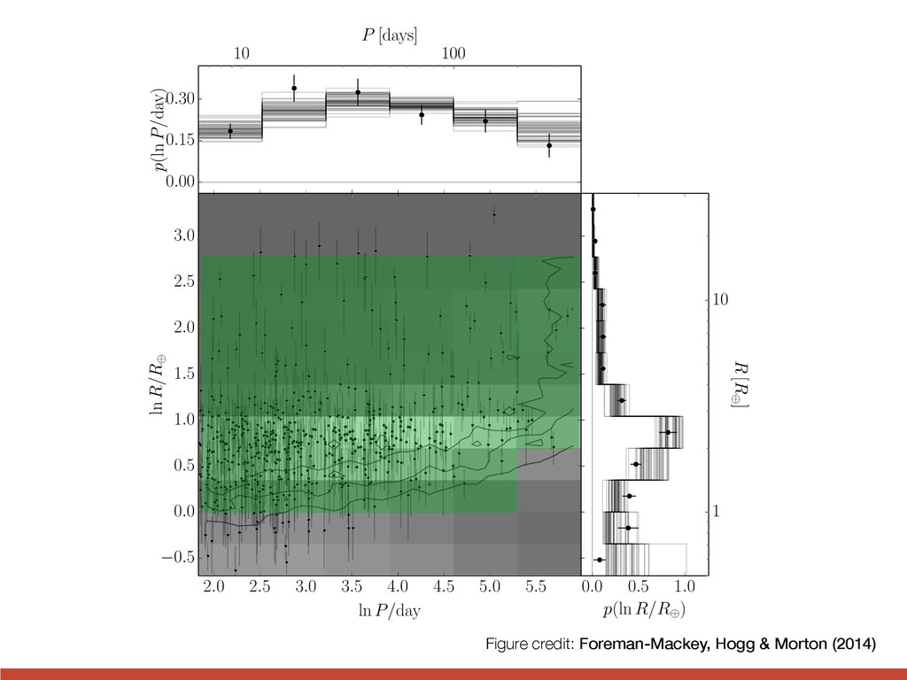
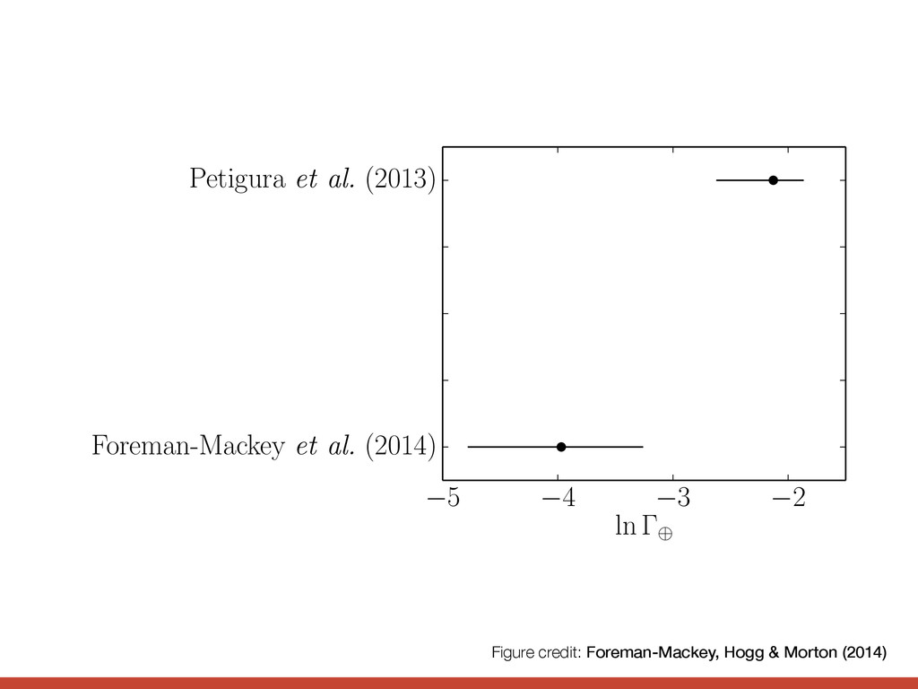
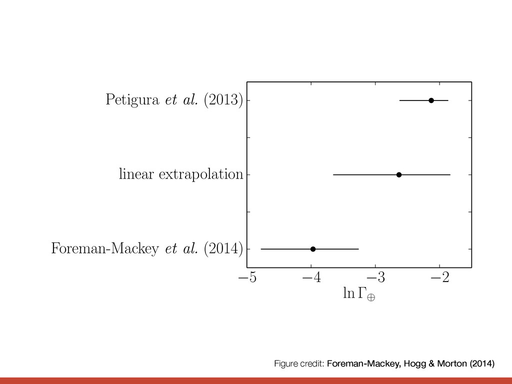
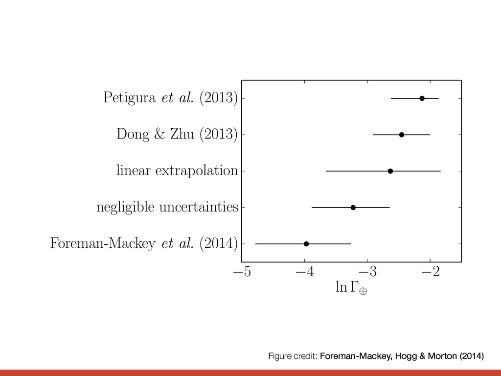
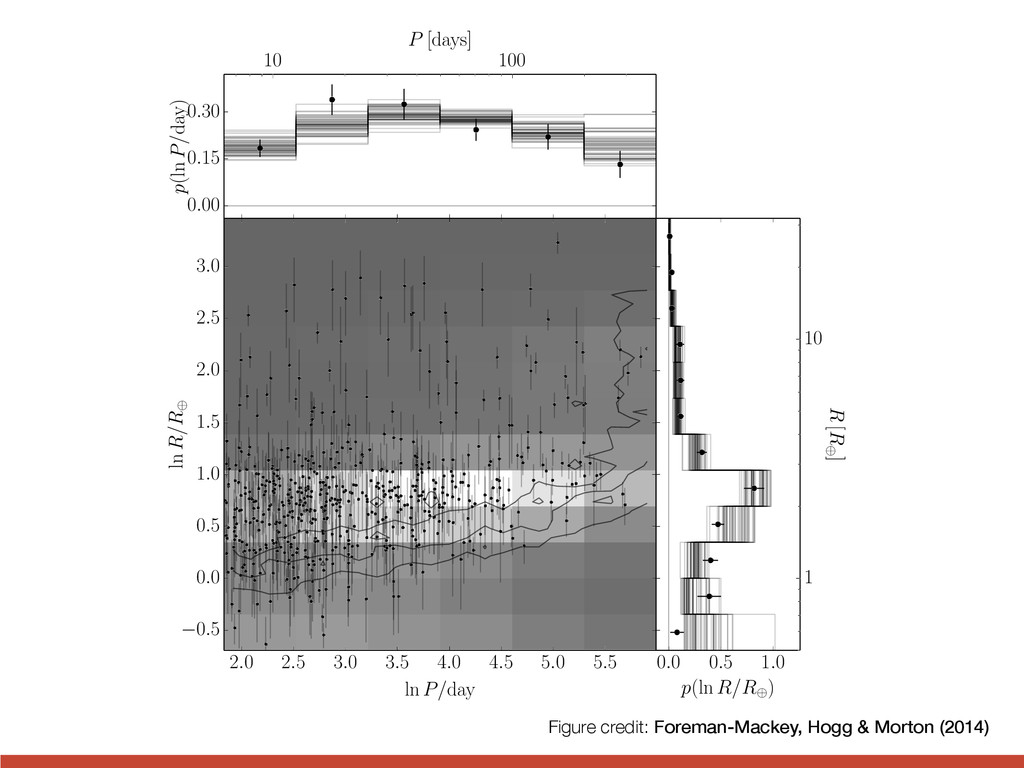
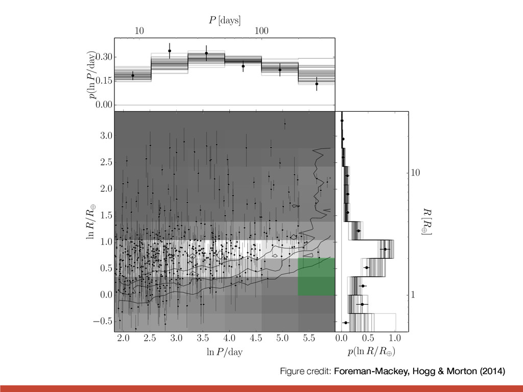
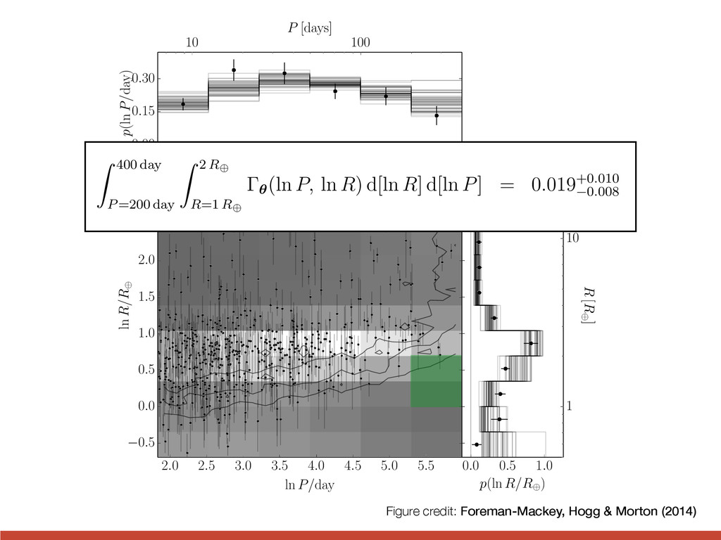
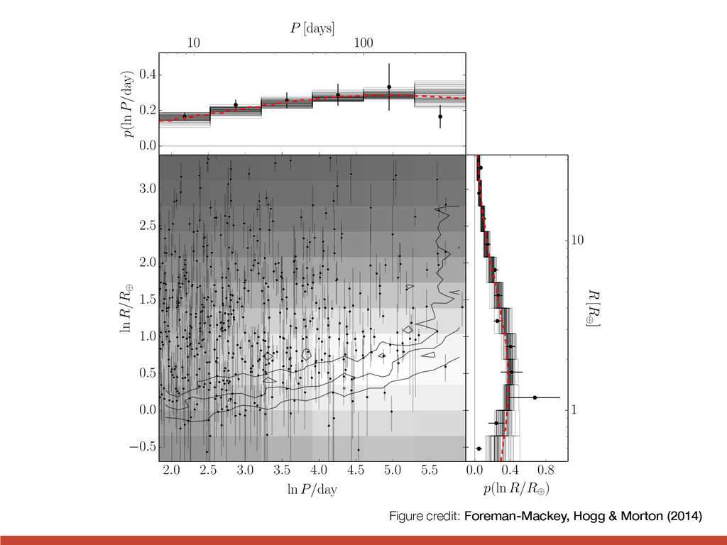
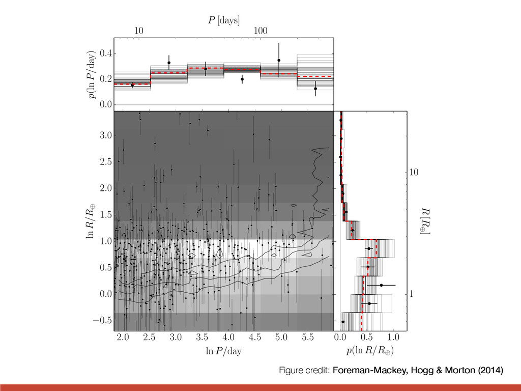
0.5 0.0 0.5 1.0 1.5 2.0 2.5 3.0 ln R/R 0.00 0.15 0.30 p(ln P/day) 0.0 0.5 1.0 p(ln R/R ) 10 100 P [days] 1 10 R [R ] Figure credit: Foreman-Mackey, Hogg & Morton (2014) nsity is exactly what Petigura’s extrapolation model predicts but, for comparison, we so integrate our inferred rate density over their choice of “Earth-like” bin (200 P/d 0 and 1 R/R < 2) to find a rate of Earth analogs. The published rate is 0.057+ Petigura et al. 2013b) and our posterior constraint is Z 400 day P=200 day Z 2 R R=1 R ✓ (ln P, ln R) d[ln R] d[ln P] = 0.019+0.010 0.008 . 9. Comparison with previous work Our inferred rate density of Earth analogs (Equation 22) is not consistent with previo ublished results. In particular, our result is completely inconsistent with the earlier r ased on exactly the same dataset (Petigura et al. 2013b). This inconsistency is du e di↵erent assumptions made but it merits some investigation. The two key di↵ere tween our analysis and previous work are (a) the form of the extrapolation function ) the presence of measurement uncertainties on the planet radii. The two main assumptions that we relax in this Article are the extrapolation
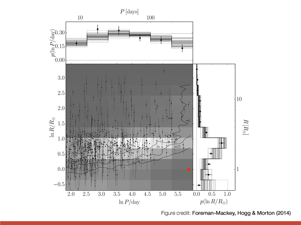
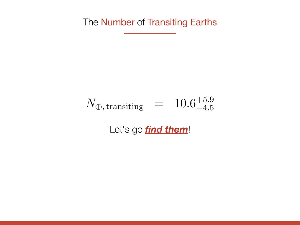
on the number of xisting Kepler dataset. If we adopt the definition of “ 013b, 200 P/day < 400 and 1 R/R < 2), and integ sity function and the geometric transit probability (Equa the expected number of Earth-like exoplanets transiting e stars chosen by Petigura et al. (2013b) is N , transiting = 10.6+5.9 4.5 ainties are only on the expectation value and don’t inc e. This is an exciting result because it means that, if we planet search pipelines to small planets orbiting on long Earth analogs in the existing data. Furthermore, because ting systems in the catalog, the True expected number of biting Sun-like stars is probably larger than the values in Let's go find them!
![Hogg, Myers, & Bovy (2010) Inferring the eccentricity distribution [1008.4146]](https://files.speakerdeck.com/presentations/715b0af011b10132168932d3f2247bb6/slide_48.jpg)