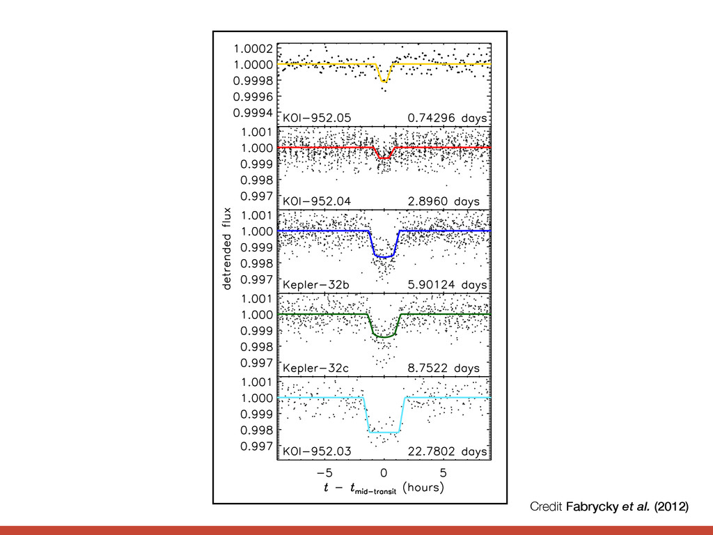
the style of figure 3. For the small inner candidate KOI-952.05, the phase is with respect to terest. The Kepler Follow-up spectra of Kepler-32: one sp servatory and one from Keck are weak due to the faintness cross correlation function be and available models is max ∼ 3900 K and ∼ 3600 K, atmospheric parameters are star is cooler than the library able. Both spectra are con sification as a cool dwarf ( [M/H]=0.172). We conserva Teff and log g with uncertain a [M/H] of 0± 0.4 based on t By comparing to the Yonse values for the stellar mass ( (0.53 ± 0.04R⊙ ) that are sli the KIC. We estimate a lum and an age of ≤ 9Gyr. Muirhead et al. (2011) h resolution IR spectrum of K a stellar Teff = 3726+73 −67 , [Fe ing their data via Padova m they inferred a considerably l We encourage further detail properties, as these have con directly affect the sizes and The probability of a star u being the actual host is only ity of a physical companion h This latter number is relative all the transit depths are sma be much larger planets hoste ically diluted. This opens up Credit Fabrycky et al. (2012)
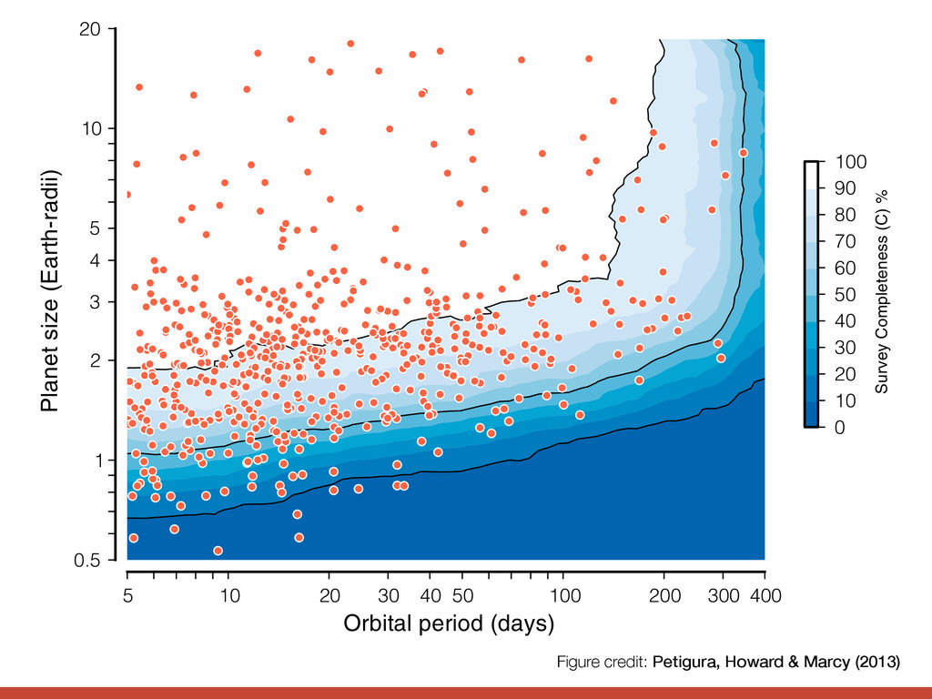
Orbital period (days) 0.5 1 2 3 4 5 10 20 Planet size (Earth-radii) 0 10 20 30 40 50 60 70 80 90 100 Survey Completeness (C) % F o d l c i p c m r o g o f Figure credit: Petigura, Howard & Marcy (2013)
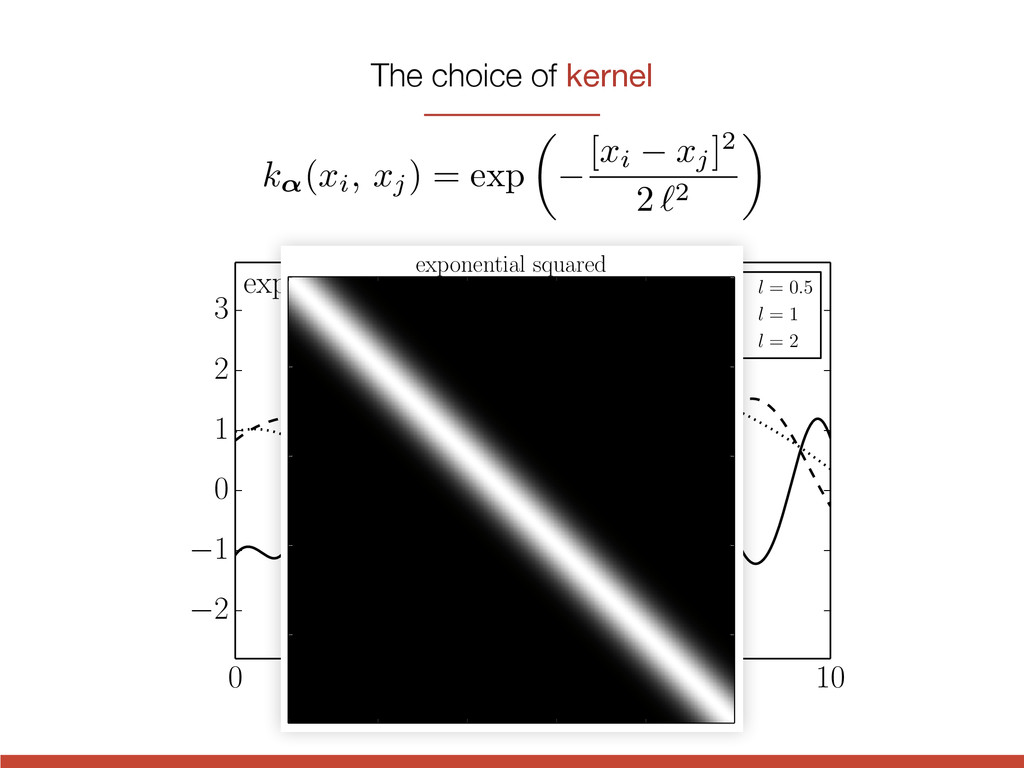
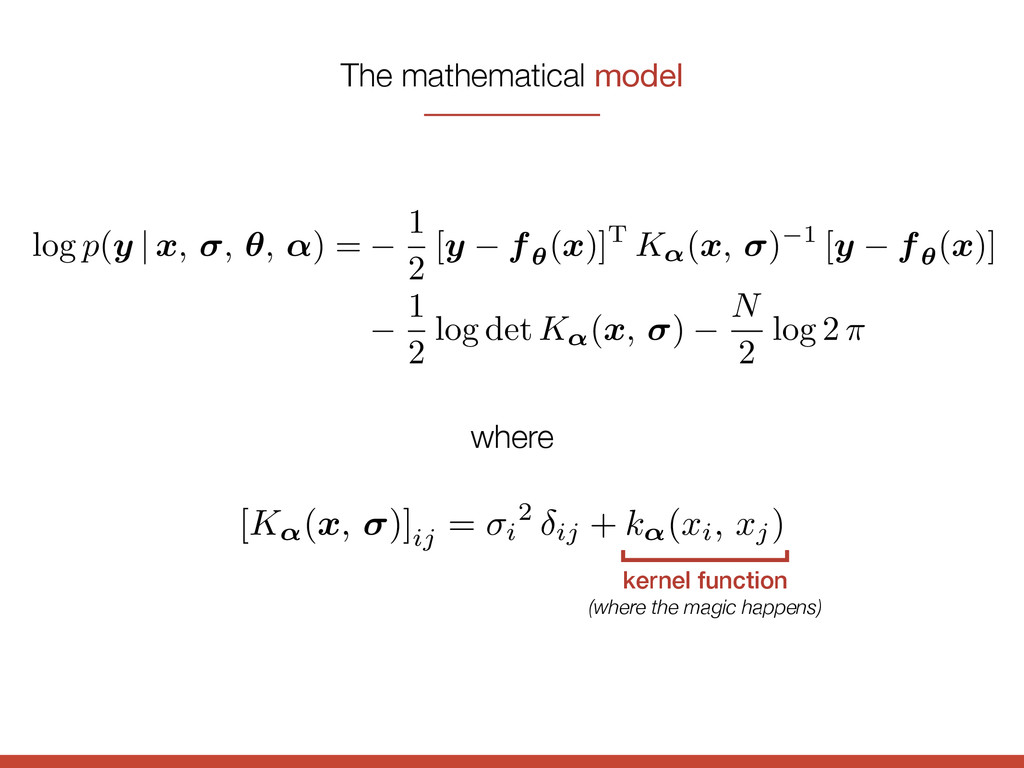
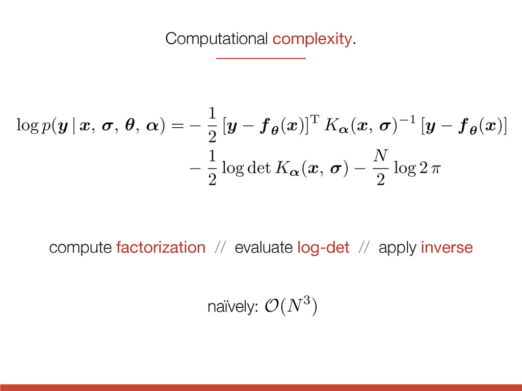
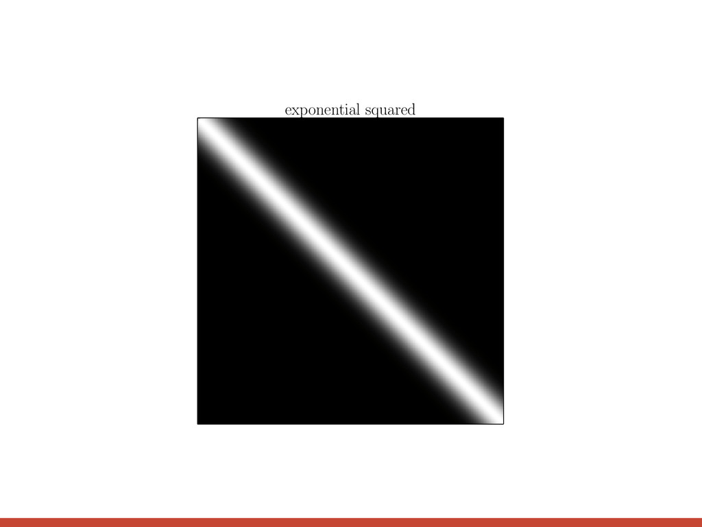
exponential squared l = 0.5 l = 1 l = 2 3 quasi-periodic l = 2, P = 3 l = 3, P = 3 l = 3, P = 1 2 1 0 1 0 2 4 6 8 10 t 2 1 0 1 2 3 quasi-periodic l = 2, P = 3 l = 3, P = 3 l = 3, P = 1 k↵(xi, xj) = exp ✓ [xi xj] 2 2 ` 2 ◆
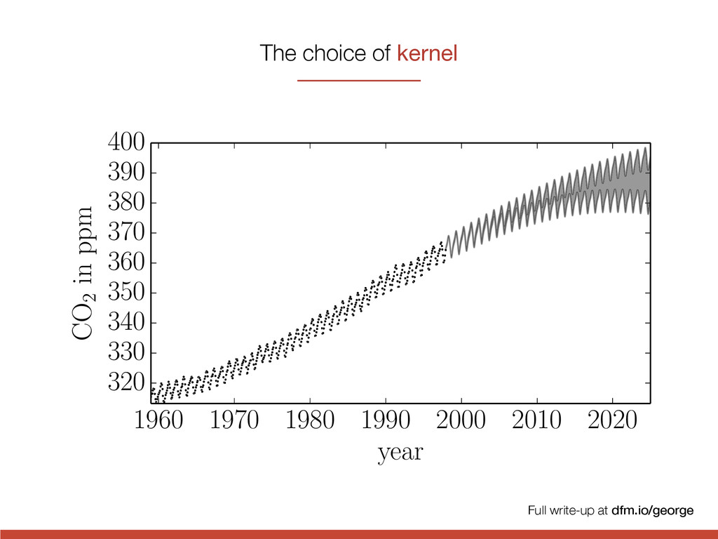
0.5 l = 1 l = 2 3 quasi-periodic l = 2, P = 3 l = 3, P = 3 l = 3, P = 1 2 1 0 1 0 2 4 6 8 10 t 2 1 0 1 2 3 quasi-periodic l = 2, P = 3 l = 3, P = 3 l = 3, P = 1 exponential squared k↵(xi, xj) = exp ✓ [xi xj] 2 2 ` 2 ◆ The choice of kernel
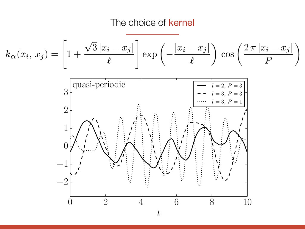
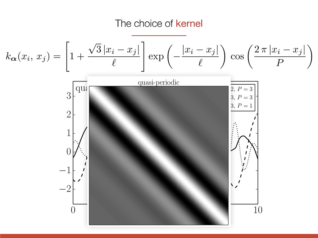
t 2 1 0 1 2 3 quasi-periodic l = 2, P = 3 l = 3, P = 3 l = 3, P = 1 k↵(xi, xj) = " 1 + p 3 | xi xj | ` # exp ✓ | xi xj | ` ◆ cos ✓ 2 ⇡ | xi xj | P ◆ The choice of kernel
t 2 1 0 1 2 3 quasi-periodic l = 2, P = 3 l = 3, P = 3 l = 3, P = 1 quasi-periodic k↵(xi, xj) = " 1 + p 3 | xi xj | ` # exp ✓ | xi xj | ` ◆ cos ✓ 2 ⇡ | xi xj | P ◆ The choice of kernel
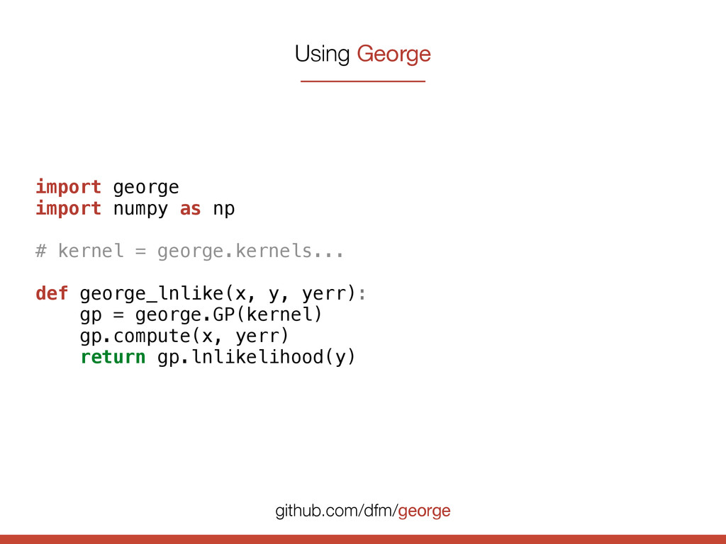
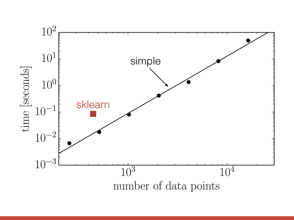
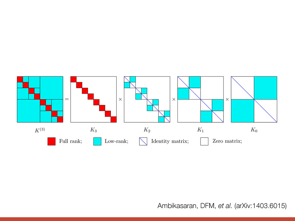
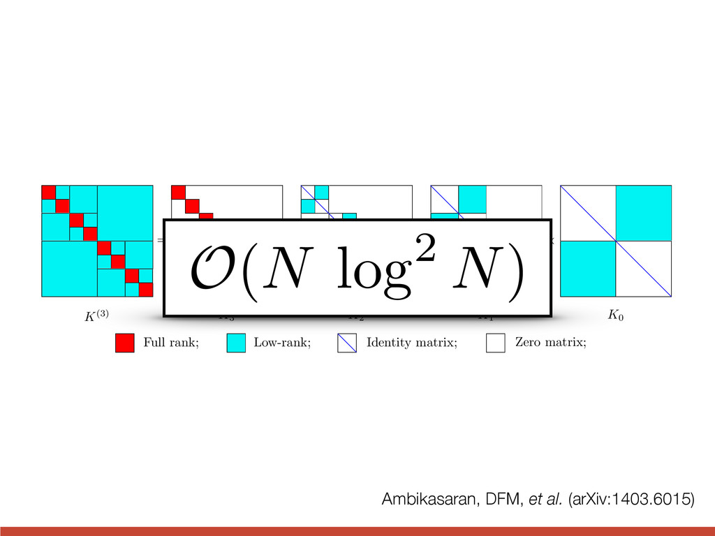
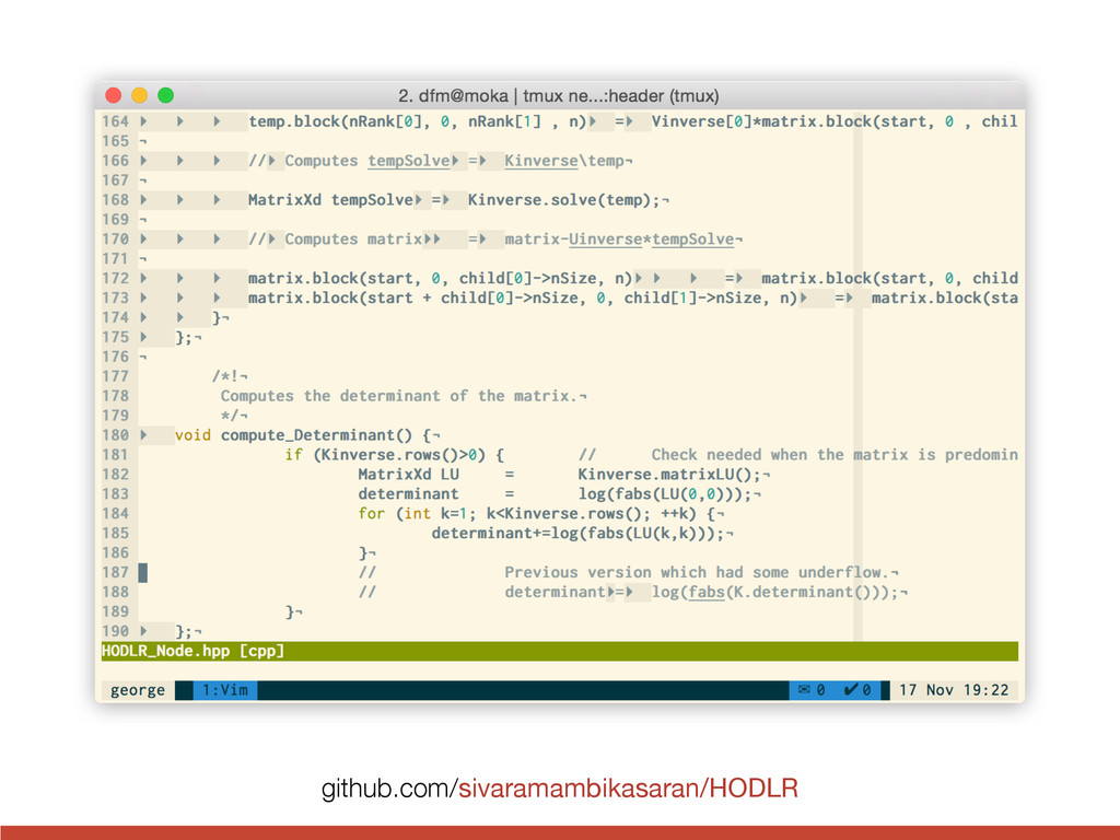
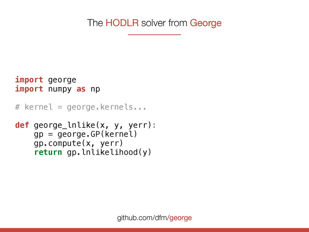
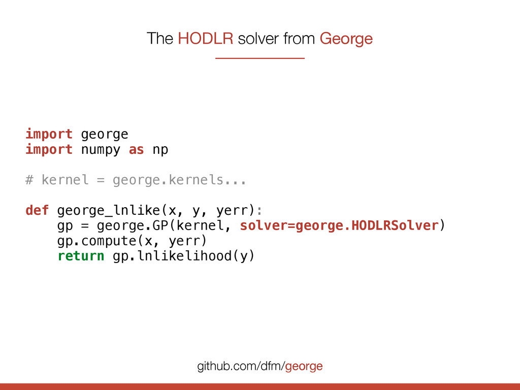
def george_lnlike(x, y, yerr): gp = george.GP(kernel, solver=george.HODLRSolver) gp.compute(x, yerr) return gp.lnlikelihood(y) The HODLR solver from George github.com/dfm/george
![1.0 0.5 0.0 0.5 1.0 time since transit [days] 100](https://files.speakerdeck.com/presentations/b55ab610555301323a2c7e116fae2d05/slide_22.jpg)
![1.0 0.5 0.0 0.5 1.0 time since transit [days] 100](https://files.speakerdeck.com/presentations/b55ab610555301323a2c7e116fae2d05/slide_32.jpg)
![1 10 100 orbital period [days] 1 10 planet radius](https://files.speakerdeck.com/presentations/b55ab610555301323a2c7e116fae2d05/slide_43.jpg)
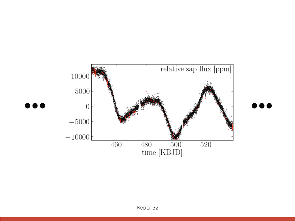
![460 480 500 520 time [days] 10000 5000 0 5000](https://files.speakerdeck.com/presentations/b55ab610555301323a2c7e116fae2d05/slide_60.jpg)
![460 480 500 520 time [days] 10000 5000 0 5000](https://files.speakerdeck.com/presentations/b55ab610555301323a2c7e116fae2d05/slide_61.jpg)
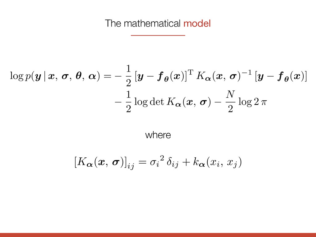
![where [ K↵( x, )]ij = i 2 ij +](https://files.speakerdeck.com/presentations/b55ab610555301323a2c7e116fae2d05/slide_63.jpg)
![References gaussianprocess.org/gpml github.com/dfm/ gp george [email protected]](https://files.speakerdeck.com/presentations/b55ab610555301323a2c7e116fae2d05/slide_87.jpg)