Insight 2 What Makes PDQ Pretty Damn Quick? Tools and Techniques First Look at PDQ From Monitoring to Modeling 3 PDQ Examples Load Balancing Multithreaded Application Web Application 4 Wrap Up Summary Resources c 2010 Performance Dynamics What’s New in PDQ? May 4, 2010 2 / 54
Quick started life in c. 1994 All computer systems contain buffers ≡ queues Performance of computers expressed as performance of queues Not a simulator, a solver ⇒ fast Solves in steady state ⇒ correct statistics Newest aspect is integration with R stats package (more later) c 2010 Performance Dynamics What’s New in PDQ? May 4, 2010 3 / 54
Harding: SWIG, Perl, python, Java Philip Feller: SWIG packaging, R, SourceForge Samuel Zallocco: PHP Stefan Parvu: Solaris testing c 2010 Performance Dynamics What’s New in PDQ? May 4, 2010 4 / 54
“All observation must be for or against some view if it is to be of any service.” Translation: All performance data should either agree or disagree with a performance model1 if it is to be of any use. 1Performance models can be constructed as: SWAG, Excel, R, Mathematica, PDQ, LoadRunner, JMeter, etc. c 2010 Performance Dynamics What’s New in PDQ? May 4, 2010 7 / 54
monitored performance data is time-series data Very difficult to discern information in such data Instantaneous time series data Time averaged information Need to transform data to provide information, e.g., PDQ c 2010 Performance Dynamics What’s New in PDQ? May 4, 2010 8 / 54
Overview Data + PDQ == Insight 2 What Makes PDQ Pretty Damn Quick? Tools and Techniques First Look at PDQ From Monitoring to Modeling 3 PDQ Examples Load Balancing Multithreaded Application Web Application 4 Wrap Up Summary Resources c 2010 Performance Dynamics What’s New in PDQ? May 4, 2010 9 / 54
Modeling Methods Two primary methods used: 1 Statistical forecasting: Apply to raw data Basically a form of trend analysis No deeper abstraction Cannot predict bottlenecks 2 Queueing analysis: Must extract queueing parameters Must create underlying abstraction Solve “analytically” or by simulation Can predict bottlenecks We will focus on queueing analysis using PDQ c 2010 Performance Dynamics What’s New in PDQ? May 4, 2010 10 / 54
Modeling Tools 1 Commercial: BMC Perform-Predict www.bmc.com TeamQuest Model www.teamquest.com HP OpenView www.hp.com HP LoadRunner www.hp.com 2 Open Freeware: Grinder, Java load-testing framework grinder.sourceforge.net/ RRDTool. Data logging and graphing system for time series data oss.oetiker.ch/rrdtool/ SimPy queueing simulator written in python simpy.sourceforge.net/ PDQ queueing solver sourceforge.net/projects/pdq-qnm-pkg/ c 2010 Performance Dynamics What’s New in PDQ? May 4, 2010 11 / 54
Queueing Models? 1 Pros: Queues are buffers. Buffers are used to hold multiple requests for shared resources. All computer systems contain buffers. Finite size in real computers, but can be unbounded in performance models (gives us a look-ahead at potenital overflow problems). Queues can formalized and calculated mathematically/programmatically. Gives them predictive power. 2 Cons: Queueing effects can be very unintuitive. The math is difficult for the non-mathematician. Commercial tools that autobuild have a server-centric view. c 2010 Performance Dynamics What’s New in PDQ? May 4, 2010 12 / 54
is Queueing Theory Difficult? Very difficult to predict optimal strategy Very difficult to choose shortest-time checkout lane Instantaneous behavior is very erratic and unpredictable Price check can kill your performance High variability or fluctuations make queueing theory difficult Theorem (Secret Weapon) Turn all fluctuations off and consider only the average behavior. That means look only at the statistical means System (checkout lane) as it appears in the long run Decorate with fluctuations (higher moments) later, if you need to c 2010 Performance Dynamics What’s New in PDQ? May 4, 2010 16 / 54
a Queue New customers arriving Serviced customers departing Queue Customer In service Server/cashier Waiting customers If arrivals and service periods are assumed to be statistically random (exponentially distributed), this kind of queue is denoted by: M/M/1 ≡ M arrival dsn / M service dsn / 1 no. servers c 2010 Performance Dynamics What’s New in PDQ? May 4, 2010 17 / 54
Metrics Symbol Metric PDQ Circuit λ Arrival rate Input Open S Service time Input Open/Closed N User load Input Closed Z Think time Input Closed R Residence time Output Open/Closed R Response time Output Open/Closed X Throughput Output Open/Closed ρ Utilization Output Open/Closed Q Queue length Output Open/Closed N∗ Optimal load Output Closed c 2010 Performance Dynamics What’s New in PDQ? May 4, 2010 18 / 54
PDQ Model in Perl #! /usr/bin/perl use pdq; # import the PDQ library as a Perl module #------------------------- INPUTS --------------------- $ArrivalRate = 0.75; # customers per minute $SeviceTime = 1.00; # seconds per customer $ServerName = "Cashier"; $Workload = "Customers"; #------------------------ PDQ Model ------------------- pdq::Init("Grocery Store Checkout"); # Initialize internal variables pdq::SetWUnit("Cust"); # Change the units pdq::SetTUnit("Min"); # used in PDQ Report # Create the PDQ service node (Cashier) $n = pdq::CreateNode($ServerName, $pdq::CEN, $pdq::FCFS); # Create the PDQ workload with arrival rate $s = pdq::CreateOpen($Workload, $ArrivalRate); # Define service rate per customer at the cashier pdq::SetDemand($ServerName, $Workload, $SeviceTime); #------------------------ OUTPUTS --------------------- pdq::Solve($pdq::CANON); pdq::Report(); # Generate a full PDQ report c 2010 Performance Dynamics What’s New in PDQ? May 4, 2010 21 / 54
Comparison of Results Symbol Metric Calculated PDQ Units R Residence time 4 4.00 minutes R Response time 4 4.00 minutes X Throughput 0.75 0.75 cust/min ρ Utilization 0.75 75.00 % Q Queue length 3 3.00 customers Whew! c 2010 Performance Dynamics What’s New in PDQ? May 4, 2010 23 / 54
PDQ Version 5.0.3 PDQ is a library of functions written in C. SWIG to Perl, Python, PHP, Java and R. PDQ-R adds queueing models to R statistical tools. Contributing maintainers: Phil Feller, Peter Harding Runs on: Cygwin, MacOS X, UNIX, Linux, Windows with ActiveState Perl, and any place you can compile C code. c 2010 Performance Dynamics What’s New in PDQ? May 4, 2010 24 / 54
PDQ Assumes Steady-State Steady state: A − C < during measurement period T Ramp up Ramp down Elapsed time Instantaneous throughput Steady-state Often don’t know where steady-state is located c 2010 Performance Dynamics What’s New in PDQ? May 4, 2010 25 / 54
SimPy vs. PyDQ Simulator stats will be off, if not run to steady state. But how long is long enough? c 2010 Performance Dynamics What’s New in PDQ? May 4, 2010 26 / 54
Estimating Service Time Parameters There are many ways to obtain service times which are critical for constructing any queueing model. 1 Performance collector databases 2 Application instrumentation 3 Java probes e.g., JXInsight 4 Little’s (microscopic) law ρ = λS: S = ρ X 5 Instruction counts from compiler: S = kiloInstrs specMIPs c 2010 Performance Dynamics What’s New in PDQ? May 4, 2010 27 / 54
== Insight 2 What Makes PDQ Pretty Damn Quick? Tools and Techniques First Look at PDQ From Monitoring to Modeling 3 PDQ Examples Load Balancing Multithreaded Application Web Application 4 Wrap Up Summary Resources c 2010 Performance Dynamics What’s New in PDQ? May 4, 2010 28 / 54
of CPUs 4 Spam detected 33901 Ham accepted 23123 Emails processed 57024 Emails per hour 2376 Per CPU/hour 594 CPU busy% 20-100 Secs per email 6 Load average (1 min) 30-105 c 2010 Performance Dynamics What’s New in PDQ? May 4, 2010 30 / 54
a load imbalance? 2 Are some servers overdriven due imbalance? 3 What is a desirable load average (Q)? 4 What should be the actual server performance? 5 How many additional servers will be needed in the next scal year to maintain current scanning performance? PDQ tells you what things should look like. GMantra 1.11: Capacity planning is about setting expectations. Even wrong expectations are better than no expectations! BTW, That’s what financial people do. c 2010 Performance Dynamics What’s New in PDQ? May 4, 2010 31 / 54
each 4-way server should be identical when balanced. Try M/M/4 model for each server. library(pdq) # Measured performance parameters cpusPerServer <- 4 emailThruput <- 2376 # emails per hour scannerTime <- 6.0 # seconds per email # Use timebase of seconds in PDQ model Init("Spam Farm Model") CreateOpen("Email", emailThruput/3600) CreateMultiNode(cpusPerServer, "spamCan", CEN, FCFS) SetDemand("spamCan", "Email", scannerTime) Solve(CANON) Report() c 2010 Performance Dynamics What’s New in PDQ? May 4, 2010 32 / 54
produces a report containing 2 sections: ****** SYSTEM Performance ******* Metric Value Unit ------ ----- ---- Workload: "Email" Number in system 100.7726 Trans Mean throughput 0.6600 Trans/Sec Response time 152.6858 Sec Stretch factor 25.4476 and ****** RESOURCE Performance ******* Metric Resource Work Value Unit ------ -------- ---- ----- ---- Throughput spamCan Email 0.0660 Trans/Sec Utilization spamCan Email 99.0000 Percent Queue length spamCan Email 100.7726 Trans Waiting line spamCan Email 96.8126 Trans Waiting time spamCan Email 146.6858 Sec Residence time spamCan Email 152.6858 Sec c 2010 Performance Dynamics What’s New in PDQ? May 4, 2010 33 / 54
4-way CPU should be 99% busy. Higher than seen on some real servers due to load imbalance Predicted load average (Q) metric is closer to 100 emails Many servers are nearly saturated now Future: Upgrade existing boxes with faster CPUS Future: Procure all new 4-way servers Theorem (Why PDQ?) PDQ is both diagnostic and predictive. c 2010 Performance Dynamics What’s New in PDQ? May 4, 2010 34 / 54
a 2-way SMP (left) with an HTT-capable (single core) processor (right). Architectural State registers (AS) can present themselves to O/S as 2 virtual processors (VPUs). [Source: Intel Developer Forum] c 2010 Performance Dynamics What’s New in PDQ? May 4, 2010 35 / 54
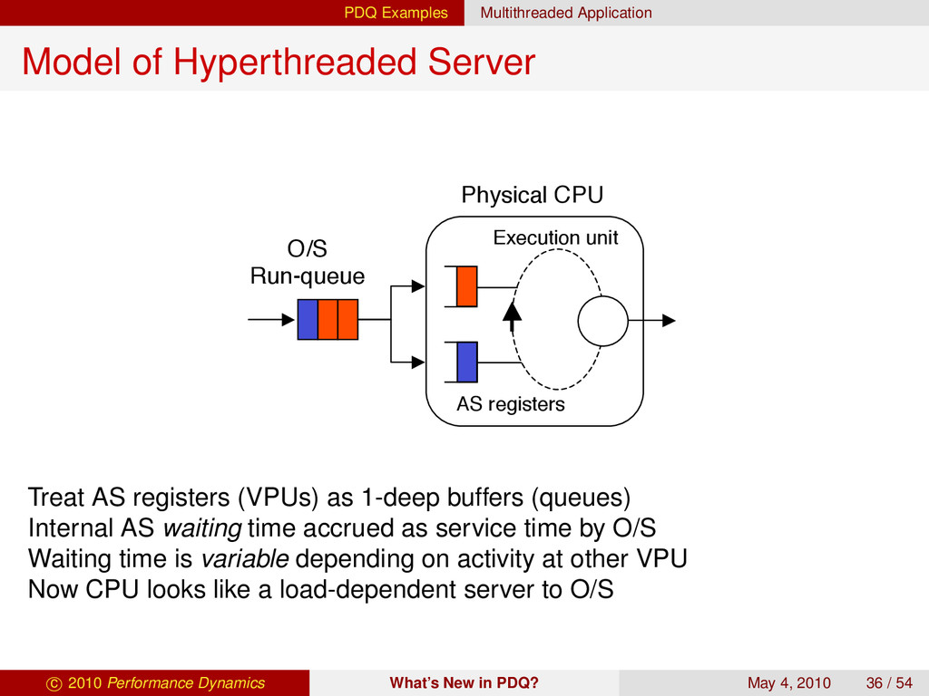
Physical CPU O/S Run-queue Execution unit Treat AS registers (VPUs) as 1-deep buffers (queues) Internal AS waiting time accrued as service time by O/S Waiting time is variable depending on activity at other VPU Now CPU looks like a load-dependent server to O/S c 2010 Performance Dynamics What’s New in PDQ? May 4, 2010 36 / 54
AS register O/S Run-queue AS registers a0 b0 cpu0 cpu1 Example: Intel Xeon processors With HTT off looks like 2 physical CPUs to O/S c 2010 Performance Dynamics What’s New in PDQ? May 4, 2010 37 / 54
AS registers O/S Run-queue AS registers a0 a1 b0 b1 cpu0 cpu1 With HTT on looks like 2 × 2 = 4 VPUs to O/S Label VPU buffers as: a0, a1, b0, b1 (Intel like) c 2010 Performance Dynamics What’s New in PDQ? May 4, 2010 39 / 54
with HTT enabled Measured with HTT ensabled 0 5 10 15 m 0.005 0.010 0.015 0.020 Throughput Previous argument supported by measurements Expected doubling of throughput is not realized Only 3/4 of expected capacity at m = 4 knee c 2010 Performance Dynamics What’s New in PDQ? May 4, 2010 40 / 54
Little’s law, Sk = ρk /X, to measured utilization (ρ) and throughput (X) data at each server tier. > # Web server > Uwebs/Xgps [1] 0.008750000 0.008541667 0.008705882 0.009500000 0.009696970 0.010319149 > # Apps server > Uapps/Xgps [1] 0.003333333 0.002708333 0.002352941 0.002300000 0.002222222 0.002340426 > # DBMS server > Udbms/Xgps [1] 0.0016666667 0.0010416667 0.0005882353 0.0005000000 0.0006060606 0.0006382979 > > Swebs<-mean(Uwebs/Xgps) > Swebs [1] 0.009252278 > Sapps [1] 0.002542876 > Sdbms [1] 0.0008401545 These calculated service times are inputs into PDQ-R model. c 2010 Performance Dynamics What’s New in PDQ? May 4, 2010 44 / 54
20 0 20 40 60 80 100 120 Clients (N) Gets/Sec X(N) Naive PDQ Model of 3-Tier WAS Measurements c 2010 Performance Dynamics What’s New in PDQ? May 4, 2010 46 / 54
achieve the same effect while maintaining Z = 0 as measured? Dws Das Ddb N clients Z = 0 ms Web Server App Server DBMS Server Requests Responses Dummy Servers Additional latency from queues whose Rk cannot exceed Rmin . Otherwise, they would introduce an artificial bottleneck. c 2010 Performance Dynamics What’s New in PDQ? May 4, 2010 48 / 54
15 20 0 20 40 60 80 100 120 Clients (N) Gets/Sec X(N) Comparison of Z = 0.03 s and 50 Dummy Delays c 2010 Performance Dynamics What’s New in PDQ? May 4, 2010 49 / 54
We accommodate this by making the service time vary with the number of request (the load N). y = 8.3437x0.0645 R2 = 0.8745 8 8.5 9 9.5 10 10.5 0 5 10 15 20 Clients (N) Service Demand Data_Dws 8.0 N^{0.085} Power (Data_Dws) Regression fit to service time data produces: S(N) = 8.0N0.085 PDQ-R load-dependent service time input: SetDemand(node1, work, 8 * nˆ(0.085) * 10ˆ(-3)) c 2010 Performance Dynamics What’s New in PDQ? May 4, 2010 50 / 54
== Insight 2 What Makes PDQ Pretty Damn Quick? Tools and Techniques First Look at PDQ From Monitoring to Modeling 3 PDQ Examples Load Balancing Multithreaded Application Web Application 4 Wrap Up Summary Resources c 2010 Performance Dynamics What’s New in PDQ? May 4, 2010 52 / 54
the Devil, models come from God. PDQ is a transformer for converting data into information. A wrong PDQ model is better than no model at all. Easy to model multi-tier systems in PDQ. Seen many PDQ models in this talk. Usually, you only need to produce one or two models. c 2010 Performance Dynamics What’s New in PDQ? May 4, 2010 53 / 54
![Wrap Up Resources My Coordinates www.perfdynamics.com perfdynamics.blogspot.com twitter.com/DrQz www.perfdynamics.com/Classes [email protected]](https://files.speakerdeck.com/presentations/8e815ca08b5f0130c5431231381090ee/slide_53.jpg)