CISC-Matchmaking-2018-Mar-6

Presentation given at the Lunchtime Matchmaking Seminar at Illinois Tech

Transcript

1. Efficient Monte Carlo Simulations Fred J. Hickernell Department of Applied Mathematics Center for Interdisciplinary Scientific Computation Illinois Institute of Technology hickernell@iit.edu mypages.iit.edu/~hickernell Supported by NSF-DMS-1522687 and DMS-1638521 (SAMSI) CISC Lunchtime Matchmaking Seminar, March 6, 2018
2. Background Save Computer Time Save User Time Summary References Problems Amenable to Monte Carlo Methods answer =                  posterior mean option price probability of an event . . .                  = Rd f(x) (x) dx Glasserman, P. Monte Carlo Methods in Financial Engineering. (Springer-Verlag, New York, 2004), Kalos, M. H. & Whitlock, P. A. Monte Carlo Methods, Volume I: Basics. (John Wiley & Sons, New York, 1986), Robert, C. P. & Casella, G. Monte Carlo Statistical Methods. Second (Springer-Verlag, New York, 2010). 2/8
3. Background Save Computer Time Save User Time Summary References Problems Amenable to Monte Carlo Methods answer =                  posterior mean option price probability of an event . . .                  = Rd f(x) (x) dx approx = 1 n n i=1 f(xi), the xi ∼ are    independent and identically distributed (IID) low discrepancy via a Markov chain    Glasserman, P. Monte Carlo Methods in Financial Engineering. (Springer-Verlag, New York, 2004), Kalos, M. H. & Whitlock, P. A. Monte Carlo Methods, Volume I: Basics. (John Wiley & Sons, New York, 1986), Robert, C. P. & Casella, G. Monte Carlo Statistical Methods. Second (Springer-Verlag, New York, 2010). 2/8
4. Background Save Computer Time Save User Time Summary References Problems Amenable to Monte Carlo Methods answer =                  posterior mean option price probability of an event . . .                  = Rd f(x) (x) dx approx = 1 n n i=1 f(xi), the xi ∼ are    independent and identically distributed (IID) low discrepancy via a Markov chain    Want to save time for computer user Glasserman, P. Monte Carlo Methods in Financial Engineering. (Springer-Verlag, New York, 2004), Kalos, M. H. & Whitlock, P. A. Monte Carlo Methods, Volume I: Basics. (John Wiley & Sons, New York, 1986), Robert, C. P. & Casella, G. Monte Carlo Statistical Methods. Second (Springer-Verlag, New York, 2010). 2/8
5. Background Save Computer Time Save User Time Summary References Problems Amenable to Monte Carlo Methods answer =                  posterior mean option price probability of an event . . .                  = Rd f(x) (x) dx approx = 1 n n i=1 f(xi), the xi ∼ are    independent and identically distributed (IID) low discrepancy via a Markov chain    Want to save time for computer user Seeking collaborators with applications Glasserman, P. Monte Carlo Methods in Financial Engineering. (Springer-Verlag, New York, 2004), Kalos, M. H. & Whitlock, P. A. Monte Carlo Methods, Volume I: Basics. (John Wiley & Sons, New York, 1986), Robert, C. P. & Casella, G. Monte Carlo Statistical Methods. Second (Springer-Verlag, New York, 2010). 2/8
6. Background Save Computer Time Save User Time Summary References Error of Monte Carlo Methods error = answer − approx = Rd f(x) (x) dx − 1 n n i=1 f(xi) = CNF(f, {xi}n i=1 ) DSC({xi}n i=1 ) VAR(f) VAR(f) 0 and measures the variation of f DSC({xi}n i=1 ) → 0 as n → ∞ and measures the discrepancy sampling distribution deviates from the distribution defining the integral CNF(f, {xi}n i=1 ) = O(1) and measures how confounded f is with the difference between the sampling and true distributions H., F. J. The Trio Identity for Quasi-Monte Carlo Error Analysis. in Monte Carlo and Quasi-Monte Carlo Methods: MCQMC, Stanford, USA, August 2016 (eds Glynn, P. & Owen, A.) to appear, arXiv:1702.01487 (Springer-Verlag, Berlin, 2018), 13–37. 3/8
7. Background Save Computer Time Save User Time Summary References Error of Monte Carlo Methods error = answer − approx = Rd f(x) (x) dx − 1 n n i=1 f(xi) = CNF(f, {xi}n i=1 ) DSC({xi}n i=1 ) VAR(f) VAR(f) 0 and measures the variation of f. Can be decreased using importance sampling or control variates. H., F. J. The Trio Identity for Quasi-Monte Carlo Error Analysis. in Monte Carlo and Quasi-Monte Carlo Methods: MCQMC, Stanford, USA, August 2016 (eds Glynn, P. & Owen, A.) to appear, arXiv:1702.01487 (Springer-Verlag, Berlin, 2018), 13–37. 3/8
8. Background Save Computer Time Save User Time Summary References Error of Monte Carlo Methods error = answer − approx = Rd f(x) (x) dx − 1 n n i=1 f(xi) = CNF(f, {xi}n i=1 ) DSC({xi}n i=1 ) VAR(f) DSC({xi}n i=1 ) → 0 as n → ∞ and measures the discrepancy sampling distribution deviates from the distribution defining the integral. O(n−1/2) for IID xi. O(n−1+ ) or better for low discrepancy xi. O(n−r) for smooth f and unequal weights for the f(xi). H., F. J. The Trio Identity for Quasi-Monte Carlo Error Analysis. in Monte Carlo and Quasi-Monte Carlo Methods: MCQMC, Stanford, USA, August 2016 (eds Glynn, P. & Owen, A.) to appear, arXiv:1702.01487 (Springer-Verlag, Berlin, 2018), 13–37. 3/8
9. Background Save Computer Time Save User Time Summary References Low Discrepancy Sampling error = Rd f(x) (x) dx − 1 n n i=1 f(xi) = CNF(f, {xi}n i=1 ) DSC({xi}n i=1 ) VAR(f) Low discrepancy sampling places the xi more evenly than IID sampling IID points Sobol’ points Integration lattice points ··· Dick, J. et al. High dimensional integration — the Quasi-Monte Carlo way. Acta Numer. 22, 133–288 (2013). 4/8
10. Background Save Computer Time Save User Time Summary References Automatically Determining the Sample Size error = Rd f(x) (x) dx − 1 n n i=1 f(xi) = CNF(f, {xi}n i=1 ) DSC({xi}n i=1 ) VAR(f) How large should n be to ensure that |error| tolerance? We have answered this question For IID sampling For low discrepancy sampling Assuming f is a Gaussian stochastic process H., F. J. et al. Guaranteed Conservative Fixed Width Confidence Intervals Via Monte Carlo Sampling. in Monte Carlo and Quasi-Monte Carlo Methods 2012 (eds Dick, J. et al.) 65 (Springer-Verlag, Berlin, 2013), 105–128. H., F. J. & Jiménez Rugama, Ll. A. Reliable Adaptive Cubature Using Digital Sequences. in Monte Carlo and Quasi-Monte Carlo Methods: MCQMC, Leuven, Belgium, April 2014 (eds Cools, R. & Nuyens, D.) 163. arXiv:1410.8615 [math.NA] (Springer-Verlag, Berlin, 2016), 367–383, Jiménez Rugama, Ll. A. & H., F. J. Adaptive Multidimensional Integration Based on Rank-1 Lattices. in Monte Carlo and Quasi-Monte Carlo Methods: MCQMC, Leuven, Belgium, April 2014 (eds Cools, R. & Nuyens, D.) 163. arXiv:1411.1966 (Springer-Verlag, Berlin, 2016), 407–422. Rathinavel, J. & H., F. J. Automatic Bayesian Cubature. in preparation. 2018+. 5/8
11. Background Save Computer Time Save User Time Summary References Option Pricing µ = fair price = Rd e−rT max   1 d d j=1 Sj − K, 0   e−zTz/2 (2π)d/2 dz ≈ $13.12 Sj = S0e(r−σ2/2)jT/d+σxj = stock price at time jT/d, x = Az, AAT = Σ = min(i, j)T/d d i,j=1 , T = 1/4, d = 13 here Abs. Error Median Worst 10% Worst 10% Tolerance Method A Error Accuracy n Time (s) 1E−2 IID diff 2E−3 100% 6.1E7 33.000 1E−2 Scr. Sobol’ PCA 1E−3 100% 1.6E4 0.040 1E−2 Scr. Sob. cont. var. PCA 2E−3 100% 4.1E3 0.019 1E−2 Bayes. Latt. PCA 2E−3 99% 1.6E4 0.051 6/8
12. Background Save Computer Time Save User Time Summary References Summary We can make Monte Carlo calculations faster through more clever sampling We can determine when to stop the calculation to meet your tolerance Theory is good, but we want more use cases to test or demonstrate its applicability. 7/8
13. Thank you Please contact me at hickernell@iit.edu These slides are available at speakerdeck.com/fjhickernell/CISC-Matchmaking-2018-Mar-6
14. Background Save Computer Time Save User Time Summary References Glasserman, P. Monte Carlo Methods in Financial Engineering. (Springer-Verlag, New York, 2004). Kalos, M. H. & Whitlock, P. A. Monte Carlo Methods, Volume I: Basics. (John Wiley & Sons, New York, 1986). Robert, C. P. & Casella, G. Monte Carlo Statistical Methods. Second (Springer-Verlag, New York, 2010). H., F. J. The Trio Identity for Quasi-Monte Carlo Error Analysis. in Monte Carlo and Quasi-Monte Carlo Methods: MCQMC, Stanford, USA, August 2016 (eds Glynn, P. & Owen, A.) to appear, arXiv:1702.01487 (Springer-Verlag, Berlin, 2018), 13–37. Dick, J., Kuo, F. & Sloan, I. H. High dimensional integration — the Quasi-Monte Carlo way. Acta Numer. 22, 133–288 (2013). H., F. J., Jiang, L., Liu, Y. & Owen, A. B. Guaranteed Conservative Fixed Width Confidence Intervals Via Monte Carlo Sampling. in Monte Carlo and Quasi-Monte Carlo 8/8
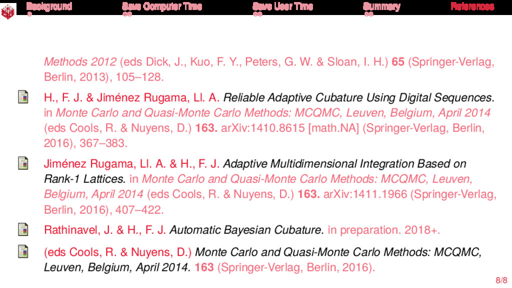
15. Background Save Computer Time Save User Time Summary References Methods 2012 (eds Dick, J., Kuo, F. Y., Peters, G. W. & Sloan, I. H.) 65 (Springer-Verlag, Berlin, 2013), 105–128. H., F. J. & Jiménez Rugama, Ll. A. Reliable Adaptive Cubature Using Digital Sequences. in Monte Carlo and Quasi-Monte Carlo Methods: MCQMC, Leuven, Belgium, April 2014 (eds Cools, R. & Nuyens, D.) 163. arXiv:1410.8615 [math.NA] (Springer-Verlag, Berlin, 2016), 367–383. Jiménez Rugama, Ll. A. & H., F. J. Adaptive Multidimensional Integration Based on Rank-1 Lattices. in Monte Carlo and Quasi-Monte Carlo Methods: MCQMC, Leuven, Belgium, April 2014 (eds Cools, R. & Nuyens, D.) 163. arXiv:1411.1966 (Springer-Verlag, Berlin, 2016), 407–422. Rathinavel, J. & H., F. J. Automatic Bayesian Cubature. in preparation. 2018+. (eds Cools, R. & Nuyens, D.) Monte Carlo and Quasi-Monte Carlo Methods: MCQMC, Leuven, Belgium, April 2014. 163 (Springer-Verlag, Berlin, 2016). 8/8