Classification, 2nd ed. John Wiley & Sons, Inc., 2001 2. S. Grossberg, “Nonlinear neural networks: Principles, mechanisms and architectures,” Neural Networks, vol. 1, no. 1, pp. 17-61, 1988. 3. M. Muhlbaier and R. Polikar, “Multiple classifiers based incremental learning algorithm for learning nonstationary environments,” in IEEE International Conference on Machine Learning and Cybernetics, 2007, pp. 3618–3623. 4. R. Elwell, “An ensemble-based computational approach for incremental learning in non-stationary environments related to schema and scaffolding-based human learning,” Master’s thesis, Rowan University, 2010. 5. J. Gao, W. Fan, J. Han, and P. S. Yu, “A general framework for mining concept-drifting data streams with skewed distributions,” in SIAM International Conference on Data Mining, 2007, pp. 203–208. 6. S. Chen and H. He, “SERA: Selectively recursive approach towards nonstationary imbalanced stream data mining,” in International Joint Conference on Neural Networks, 2009, pp. 552–529. 7. S. Chen, H. He, K. Li, and S. Sesai, “MuSERA: Multiple selectively recursive approach towards imbalanced stream data mining,” in International Joint Conference on Neural Networks, 2010, pp. 2857–2864. 8. S. Chen and H. He, “Towards incremental learning of nonstationary imbalanced data streams: a multiple selectively recursive approach,” Evolving Systems, in press, 2011. 9. R. Polikar, L. Udpa, S.S. Udpa and V. Honavar, “Learn++: an incremental learning algorithm for supervised neural networks,” IEEE Transactions on Systems, Man and Cybernetics, vol. 31, no. 4, pp. 497–508, 2001. 10. G. Ditzler, N. V. Chawla, and R. Polikar, “An incremental learning algorithm for nonstationary environments and class imbalance,” in International Conference on Pattern Recognition, 2010, pp. 2997–3000. 11. G. Ditzler and R. Polikar, “An incremental learning framework for concept drift and class imbalance,” in International Joint Conference on Neural Networks, 2010, pp. 736–473. 12. C. Li, “Classifying imbalanced data using a bagging ensemble variation (BEV),” in ACMSE, 2007, pp. 203–208. 13. N. V. Chawla, A. Lazarevic, L. O. Hall and K. W. Bowyer, “SMOTEBoost: Improving prediction of the minority class in boosting,” in 7th European Conference on Principles and Practice of Knowledge Discovery in Databases, 2003, pp. 1–10. 14. H. Guo and H. L. Viktor, “Learning from imbalanced data sets with boosting and data generation: The Databoost-IM approach,” Sigkdd Explorations, vol. 6, no. 1, pp. 30–39, 2004. 15. S. Chen and H. He, “RAMOBoost: Ranked Minority Oversampling in Boosting,” IEEE Transactions on Neural Networks, vol. 21, no. 10, pp. 1624-1642, 2010. 16. T. Fawcett, “An introduction to ROC analysis,” Pattern Recognition Letters, vol. 27, pp. 861–874, 2006. 17. W. N. Street and Y. Kim, “A streaming ensemble algorithm (SEA) for large scale classification,” in Proceedings to the 7th ACM SIGKDD International Conference on Knowledge Discovery & Data Mining, 2001, pp. 377–382. 18. J. Demšar, “Statistical comparisons of classifiers over multiple data sets,” Journal of Machine Learning Research, vol. 7, pp. 1– 30, 2006. 19. N. V. Chawla, K. W. Bowyer, L. O. Hall, and W. P. Kegelmeyer, “SMOTE: Synthetic minority over-sampling technique,” Journal of Artificial Intelligence Research, vol. 16, pp. 321–357, 2002. Introduction Approach Experiments Conclusions
![SMOTE • Synthetic Minority Over-sampling TEchnique [19] o Generate “synthetic”](https://files.speakerdeck.com/presentations/a6a56360ccc1013015c63a0a82892cf4/slide_15.jpg)
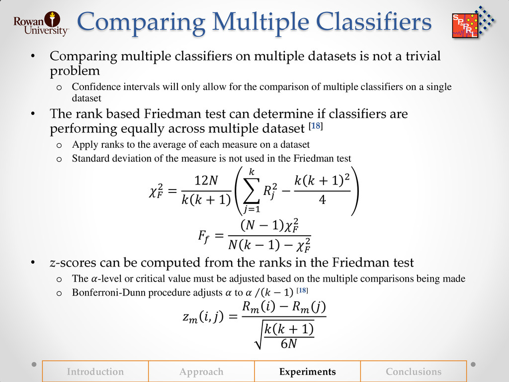
![Friedman Test Results Hypothesis test comparing NIE(fm) [◊] and CDS](https://files.speakerdeck.com/presentations/a6a56360ccc1013015c63a0a82892cf4/slide_43.jpg)