Joint modelling of longitudinal and time-to-event data: recent extensions

A half-day workshop presented at the University of Liverpool, London Campus.

Transcript

1. Introduction Competing risks Multivariate data Clinical applications Meta-analysis Dynamic prediction Software References Joint modelling of longitudinal and time-to-event data: recent extensions Graeme L. Hickey1, Pete Philipson2, Maria E. Sudell1, Ruwanthi-Kolamunnage-Dona1 1Department of Biostatistics, University of Liverpool, UK 2Mathematics, Physics and Electrical Engineering, University of Northumbria, UK graeme.hickey@liverpool.ac.uk 25th April 2018 1/165
2. Introduction Competing risks Multivariate data Clinical applications Meta-analysis Dynamic prediction Software References An MRC funded workshop 2/165
3. Introduction Competing risks Multivariate data Clinical applications Meta-analysis Dynamic prediction Software References Timetable Time What Who 1100 – 1130 Introduction to joint modelling P. Philipson 1130 – 1145 Extension I: Competing risks R. Kolamunnage-Dona 1145 – 1210 Extension II: Multiple longitudinal outcomes G. L. Hickey 1210 – 1225 Applications in clinical research R. Kolamunnage-Dona 1225 – 1245 Extension III: Meta-analysis M. E. Sudell 1245 – 1300 Extension IV: Dynamic prediction G. L. Hickey 1300 – 1345 Lunch 1345 – 1630 Software practical 3/165
4. Introduction Competing risks Multivariate data Clinical applications Meta-analysis Dynamic prediction Software References Practical information References are given in the bibliography (slide 162 – onwards) Time for questions during lunch or software sessions1 1Please find myself, Ruwanthi, Pete, or Maria 4/165
5. Introduction Competing risks Multivariate data Clinical applications Meta-analysis Dynamic prediction Software References Introduction 5/165
6. Introduction Competing risks Multivariate data Clinical applications Meta-analysis Dynamic prediction Software References Motivation Many scientific investigations follow-up subjects repeatedly over time and generate both Longitudinal measurement data Repeated measurements of a response variable at a number of time points, e.g. biomarker measurements quality of life assessments Event history data Time(s) to (possibly recurrent or) terminating events, e.g. time to death time to study withdrawal / dropout 6/165
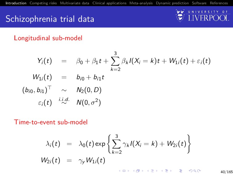
7. Introduction Competing risks Multivariate data Clinical applications Meta-analysis Dynamic prediction Software References Schizophrenia trial data A placebo-controlled randomized clinical trial of drug treatments for schizophrenia (Henderson et al. 2000) In the original trial there were three treatment arms: placebo, standard, and novel compound (subdivided into 4 dosages) We will analyse a sample of 150 patients (50 patients per treatment arm) 7/165
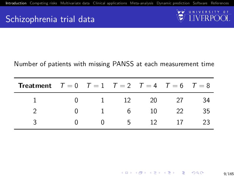
8. Introduction Competing risks Multivariate data Clinical applications Meta-analysis Dynamic prediction Software References Schizophrenia trial data The repeated measurement outcome was a questionnaire-based measure, the positive and negative symptom score (PANSS) — a measure of psychiatric disorder — taken at weeks 0, 1, 2, 4, 6 and 8 following randomization The time-to-event outcome was defined as withdrawal from the study due to ‘inadequate response’ Failure to complete the trial protocol for other reasons, unrelated to the subject’s mental state, are regarded here as uninformatively missing values, rather than as dropouts 8/165
9. Introduction Competing risks Multivariate data Clinical applications Meta-analysis Dynamic prediction Software References Schizophrenia trial data Number of patients with missing PANSS at each measurement time Treatment T = 0 T = 1 T = 2 T = 4 T = 6 T = 8 1 0 1 12 20 27 34 2 0 1 6 10 22 35 3 0 0 5 12 17 23 9/165
10. Introduction Competing risks Multivariate data Clinical applications Meta-analysis Dynamic prediction Software References Focus Depending of the focus of the research question, we might use either Separate analyses of one or more of the outcomes Joint analysis of the different outcomes 10/165
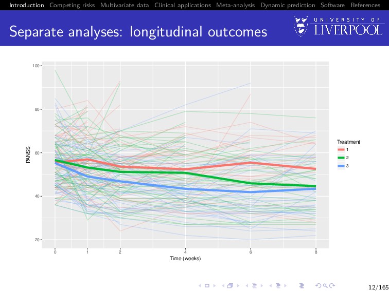
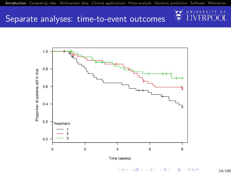
11. Introduction Competing risks Multivariate data Clinical applications Meta-analysis Dynamic prediction Software References Separate analyses Is the average PANSS score trajectory different between treatment groups? Does patient dropout differ between treatment group? 11/165
12. Introduction Competing risks Multivariate data Clinical applications Meta-analysis Dynamic prediction Software References Separate analyses: longitudinal outcomes 20 40 60 80 100 0 1 2 4 6 8 Time (weeks) PANSS Treatment 1 2 3 12/165
13. Introduction Competing risks Multivariate data Clinical applications Meta-analysis Dynamic prediction Software References Separate analyses: longitudinal outcomes Linear mixed effects model with treatment Xi ∈ {1, 2, 3} Yi (t) = (β0 + bi0) + (β1 + bi1)t + β2I(Xi = 2)t + β3I(Xi = 3)t + εi (t) (bi0, bi1) ∼ N2(0, D) εi (t) i.i.d. ∼ N(0, σ2) 13/165
14. Introduction Competing risks Multivariate data Clinical applications Meta-analysis Dynamic prediction Software References Separate analyses: longitudinal outcomes Linear mixed effects model with treatment Xi ∈ {1, 2, 3} Yi (t) = (β0 + bi0) + (β1 + bi1)t + β2I(Xi = 2)t + β3I(Xi = 3)t + εi (t) (bi0, bi1) ∼ N2(0, D) εi (t) i.i.d. ∼ N(0, σ2) Fitting the model in R Using nlme::lme()2, we get: ˆ β2 = −1.4 (SE = 0.46) and ˆ β3 = −2.1 (SE = 0.45) 2See Pinheiro and Bates (2000) 13/165
15. Introduction Competing risks Multivariate data Clinical applications Meta-analysis Dynamic prediction Software References Separate analyses: time-to-event outcomes 0 2 4 6 8 0.0 0.2 0.4 0.6 0.8 1.0 Time (weeks) Proportion of patients still in trial Treatment 1 2 3 14/165
16. Introduction Competing risks Multivariate data Clinical applications Meta-analysis Dynamic prediction Software References Separate analyses: time-to-event outcomes Cox proportional hazards model with treatment Xi ∈ {1, 2, 3} λi (t) = lim dt→0 P(t ≤ T < t + dt | T ≥ t) dt = λ0(t) exp{γ2I(Xi = 2) + γ3I(Xi = 3)} with λ0(t) left unspecified 15/165
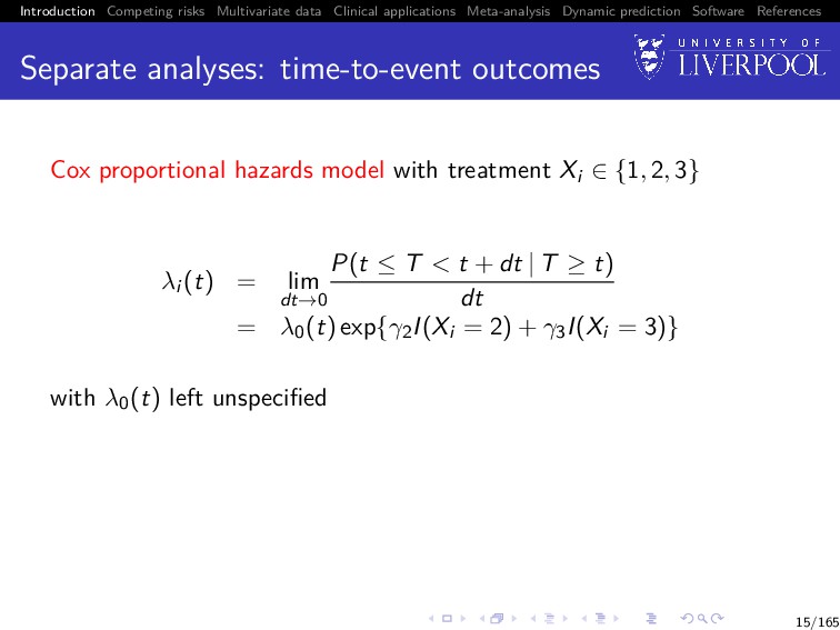
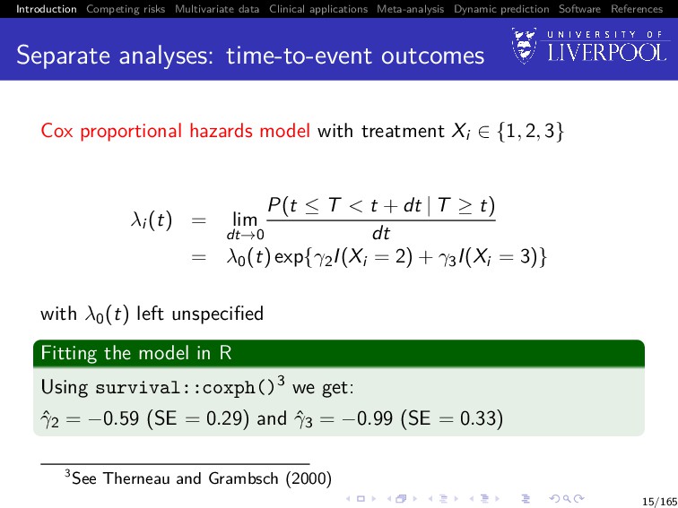
17. Introduction Competing risks Multivariate data Clinical applications Meta-analysis Dynamic prediction Software References Separate analyses: time-to-event outcomes Cox proportional hazards model with treatment Xi ∈ {1, 2, 3} λi (t) = lim dt→0 P(t ≤ T < t + dt | T ≥ t) dt = λ0(t) exp{γ2I(Xi = 2) + γ3I(Xi = 3)} with λ0(t) left unspecified Fitting the model in R Using survival::coxph()3 we get: ˆ γ2 = −0.59 (SE = 0.29) and ˆ γ3 = −0.99 (SE = 0.33) 3See Therneau and Grambsch (2000) 15/165
18. Introduction Competing risks Multivariate data Clinical applications Meta-analysis Dynamic prediction Software References Joint analysis It is not clear whether the apparent decrease in PANSS profiles reflects 1 a genuine change over time, or 2 an artefact caused by selective drop-out, with patients with high (worse) PANSS values being less likely to complete the trial 16/165
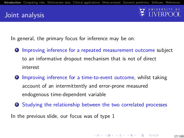
19. Introduction Competing risks Multivariate data Clinical applications Meta-analysis Dynamic prediction Software References Joint analysis In general, the primary focus for inference may be on: 1 Improving inference for a repeated measurement outcome subject to an informative dropout mechanism that is not of direct interest 2 Improving inference for a time-to-event outcome, whilst taking account of an intermittently and error-prone measured endogenous time-dependent variable 3 Studying the relationship between the two correlated processes In the previous slide, our focus was of type 1 17/165
20. Introduction Competing risks Multivariate data Clinical applications Meta-analysis Dynamic prediction Software References Joint analysis Interest might also be about 1 Prediction4: given the measurement data for a patient up to time t, what is their survivorship distribution at time s > t? 2 Surrogacy5: when the clinical event is rare or takes a long time to reach, we want to use more easily measured markers as a substitute, which can usually lead to substantial sample size reduction and shorter trial duration. In other words, is [T | X, Y ] = [T|Y ]? 4e.g. Andrinopoulou et al. (2017) 5e.g. Xu and Zeger (2001) 18/165
21. Introduction Competing risks Multivariate data Clinical applications Meta-analysis Dynamic prediction Software References Joint analysis What methods can we use to answer these sorts of questions? Separate analyses: simply ignore the association Naive models: Cox regression with time-varying covariate(s) assuming last-value carried forward Two-stage models: the LMM is first fitted separately, and the best linear unbiased predictors (BLUPS) of the random effects extracted and included in a time-varying covariate survival model Pattern mixture or selection models: factorize the joint distribution as either [Y , T] = [T] × [Y | T] = [Y ] × [T | Y ] Landmarking: refitting the survival model at sequential follow-up times conditional on subjects still in the risk set Joint models: focus of today’s workshop 19/165
22. Introduction Competing risks Multivariate data Clinical applications Meta-analysis Dynamic prediction Software References Univariate joint models 20/165
23. Introduction Competing risks Multivariate data Clinical applications Meta-analysis Dynamic prediction Software References A brief history Originally motivated by AIDS research in which a biomarker such as CD4 lymphocyte count is determined intermittently and its relationship with time to seroconversion or death is of interest Seminal articles by Wulfsohn and Tsiatis (1997) and Henderson et al. (2000) contributed to a rapidly growing research field As of 2015: > 200 methodological papers and > 60 clinical applications of joint models 21/165
24. Introduction Competing risks Multivariate data Clinical applications Meta-analysis Dynamic prediction Software References Conceptual principle Covariate data Longitudinal outcomes data Random effects ! 22/165
25. Introduction Competing risks Multivariate data Clinical applications Meta-analysis Dynamic prediction Software References Conceptual principle Covariate data Time-to-event outcomes data Frailties !" 22/165
26. Introduction Competing risks Multivariate data Clinical applications Meta-analysis Dynamic prediction Software References Conceptual principle Covariate data Time-to-event outcomes data Frailties !" Longitudinal outcomes data Random effects # 22/165
27. Introduction Competing risks Multivariate data Clinical applications Meta-analysis Dynamic prediction Software References Conceptual principle Covariate data Time-to-event outcomes data Frailties !" Longitudinal outcomes data Random effects # ! $ 22/165
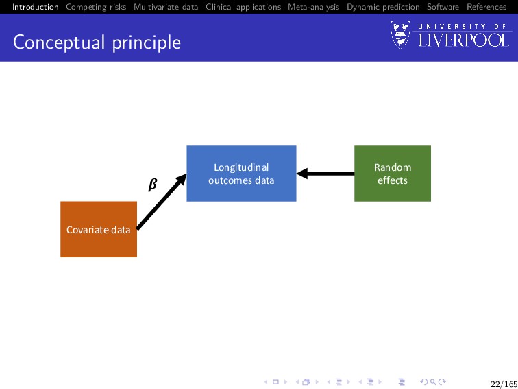
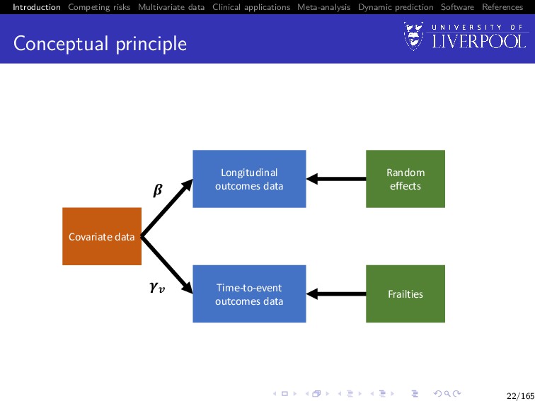
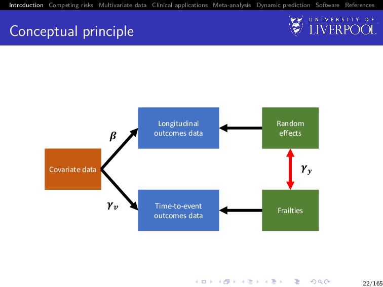
28. Introduction Competing risks Multivariate data Clinical applications Meta-analysis Dynamic prediction Software References Data For each subject i = 1, . . . , n, we observe An ni -vector of observed longitudinal measurements for the longitudinal outcome: yi = (yi1, . . . , yini ) Observation times tij for j = 1, . . . , ni , which can differ between subjects (Ti , δi ), where Ti = min(T∗ i , Ci ), where T∗ i is the true event time, Ci corresponds to a potential right-censoring time, and δi is the failure indicator equal to 1 if the failure is observed (T∗ i ≤ Ci ) and 0 otherwise 23/165
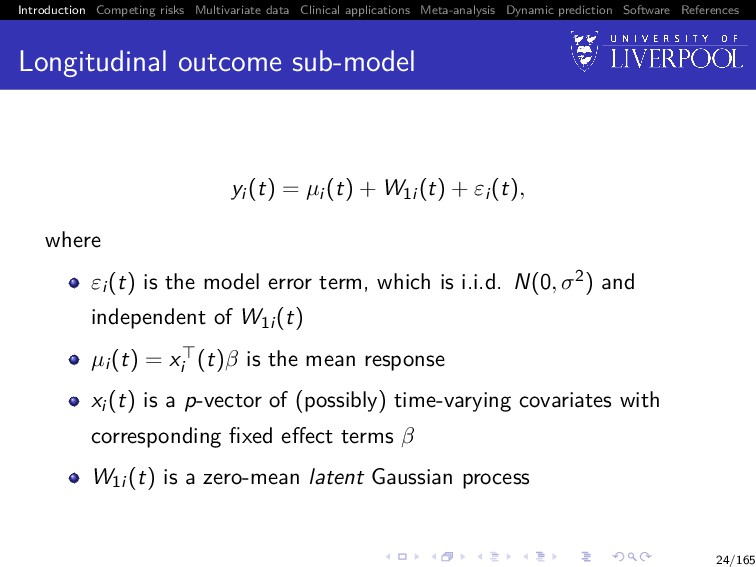
29. Introduction Competing risks Multivariate data Clinical applications Meta-analysis Dynamic prediction Software References Longitudinal outcome sub-model yi (t) = µi (t) + W1i (t) + εi (t), where εi (t) is the model error term, which is i.i.d. N(0, σ2) and independent of W1i (t) µi (t) = xi (t)β is the mean response xi (t) is a p-vector of (possibly) time-varying covariates with corresponding fixed effect terms β W1i (t) is a zero-mean latent Gaussian process 24/165
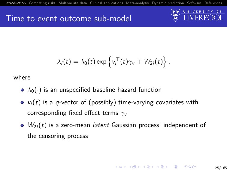
30. Introduction Competing risks Multivariate data Clinical applications Meta-analysis Dynamic prediction Software References Time to event outcome sub-model λi (t) = λ0(t) exp vi (t)γv + W2i (t) , where λ0(·) is an unspecified baseline hazard function vi (t) is a q-vector of (possibly) time-varying covariates with corresponding fixed effect terms γv W2i (t) is a zero-mean latent Gaussian process, independent of the censoring process 25/165
31. Introduction Competing risks Multivariate data Clinical applications Meta-analysis Dynamic prediction Software References Association structure W1(t) Following Laird and Ware (1982): W1i (t) = zi (t)bi , with bi ∼ N(0, D) 26/165
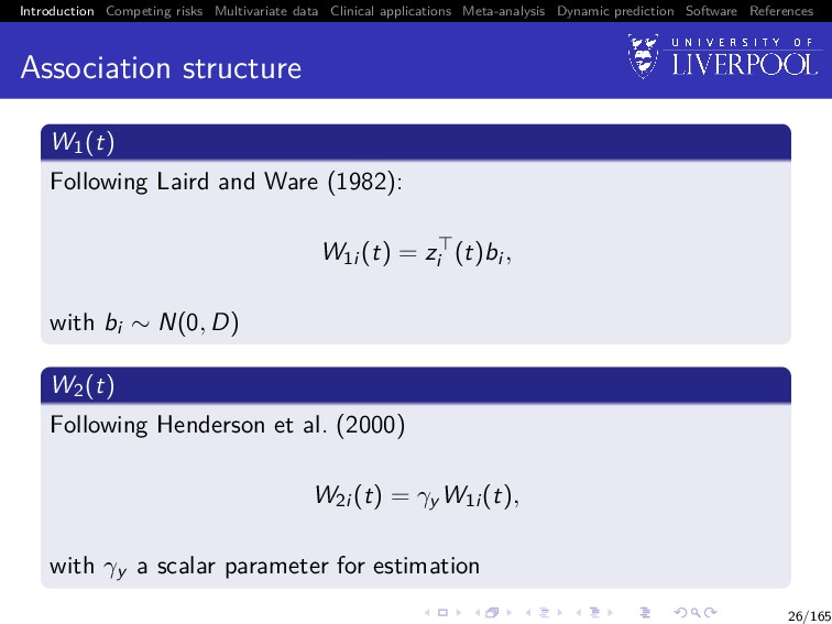
32. Introduction Competing risks Multivariate data Clinical applications Meta-analysis Dynamic prediction Software References Association structure W1(t) Following Laird and Ware (1982): W1i (t) = zi (t)bi , with bi ∼ N(0, D) W2(t) Following Henderson et al. (2000) W2i (t) = γy W1i (t), with γy a scalar parameter for estimation 26/165
33. Introduction Competing risks Multivariate data Clinical applications Meta-analysis Dynamic prediction Software References Association structure: extensions Henderson et al. (2000) proposed several extensions: 1 W1i (t) = zi (t)bi + V1i (t), where V1i (t) is a stationary Gaussian process with zero mean, variance σ2 v1 , and correlation function r1(u) = cov {V1i (t), V1i (t − u)} /σ2 v1 2 W2(t) = γy1 bi + γy2W1i (t) + θi , where γy = (γy1 , γy2) is a vector of association parameters, and θi is a frailty term independent from the longitudinal data 27/165
34. Introduction Competing risks Multivariate data Clinical applications Meta-analysis Dynamic prediction Software References Association structure: alternatives Many other proposals for association structures in the literature: Current value parameterisation: W2i (t) = γy {µi (t) + W1i (t)} Random effects parameterisation: W2i (t) = γy1 bi Bivariate distribution: (W1i , W2i ) ∼ N(0, Ω) Random-slopes parameterisation: W2i (t) = γy1 {µi (t) + W1i (t)} + γy2 ∂ ∂t {µi (t) + W1i (t)} . . . 28/165
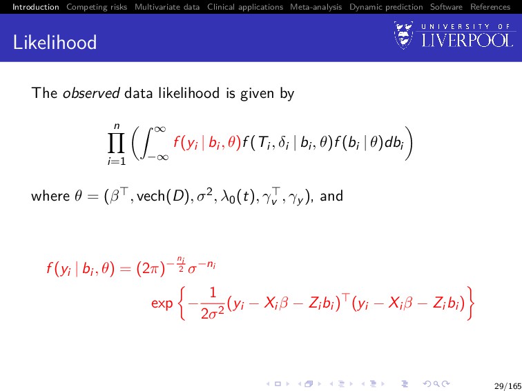
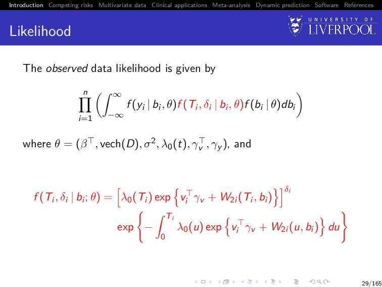
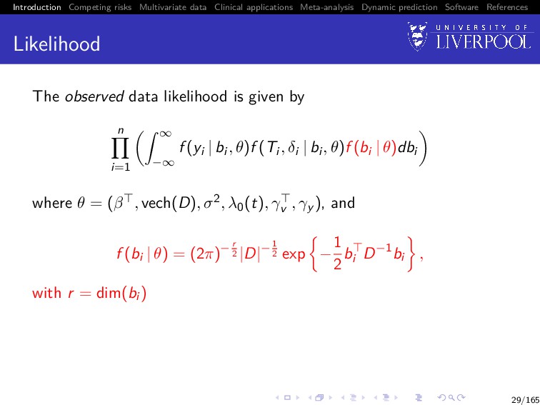
35. Introduction Competing risks Multivariate data Clinical applications Meta-analysis Dynamic prediction Software References Likelihood The observed data likelihood is given by n i=1 ∞ −∞ f (yi | bi , θ)f (Ti , δi | bi , θ)f (bi | θ)dbi where θ = (β , vech(D), σ2, λ0(t), γv , γy ) 29/165
36. Introduction Competing risks Multivariate data Clinical applications Meta-analysis Dynamic prediction Software References Likelihood The observed data likelihood is given by n i=1 ∞ −∞ f (yi | bi , θ)f (Ti , δi | bi , θ)f (bi | θ)dbi where θ = (β , vech(D), σ2, λ0(t), γv , γy ), and f (yi | bi , θ) = (2π)−ni 2 σ−ni exp − 1 2σ2 (yi − Xi β − Zi bi ) (yi − Xi β − Zi bi ) 29/165
37. Introduction Competing risks Multivariate data Clinical applications Meta-analysis Dynamic prediction Software References Likelihood The observed data likelihood is given by n i=1 ∞ −∞ f (yi | bi , θ)f (Ti , δi | bi , θ)f (bi | θ)dbi where θ = (β , vech(D), σ2, λ0(t), γv , γy ), and f (Ti , δi | bi ; θ) = λ0(Ti ) exp vi γv + W2i (Ti , bi ) δi exp − Ti 0 λ0(u) exp vi γv + W2i (u, bi ) du 29/165
38. Introduction Competing risks Multivariate data Clinical applications Meta-analysis Dynamic prediction Software References Likelihood The observed data likelihood is given by n i=1 ∞ −∞ f (yi | bi , θ)f (Ti , δi | bi , θ)f (bi | θ)dbi where θ = (β , vech(D), σ2, λ0(t), γv , γy ), and f (bi | θ) = (2π)− r 2 |D|−1 2 exp − 1 2 bi D−1bi , with r = dim(bi ) 29/165
39. Introduction Competing risks Multivariate data Clinical applications Meta-analysis Dynamic prediction Software References Estimation Multiple approaches have been considered over the years: Markov chain Monte Carlo (MCMC) Direct likelihood maximisation (e.g. Newton-methods) Generalised estimating equations EM algorithm (treating the random effects as missing data) . . . 30/165
40. Introduction Competing risks Multivariate data Clinical applications Meta-analysis Dynamic prediction Software References EM algorithm (Dempster et al. 1977) E-step. At the m-th iteration, we compute the expected log-likelihood of the complete data conditional on the observed data and the current estimate of the parameters. Q(θ | ˆ θ(m)) = n i=1 E log f (yi , Ti , δi , bi | θ) , = n i=1 ∞ −∞ log f (yi , Ti , δi , bi | θ) f (bi | Ti , δi , yi ; ˆ θ(m))dbi 31/165
41. Introduction Competing risks Multivariate data Clinical applications Meta-analysis Dynamic prediction Software References EM algorithm (Dempster et al. 1977) E-step. At the m-th iteration, we compute the expected log-likelihood of the complete data conditional on the observed data and the current estimate of the parameters. Q(θ | ˆ θ(m)) = n i=1 E log f (yi , Ti , δi , bi | θ) , = n i=1 ∞ −∞ log f (yi , Ti , δi , bi | θ) f (bi | Ti , δi , yi ; ˆ θ(m))dbi M-step. We maximise Q(θ | ˆ θ(m)) with respect to θ. namely, ˆ θ(m+1) = arg max θ Q(θ | ˆ θ(m)) 31/165
42. Introduction Competing risks Multivariate data Clinical applications Meta-analysis Dynamic prediction Software References M-step: closed form estimators ˆ λ0(t) = n i=1 δi I(Ti = t) n i=1 E exp vi γv + W2i (t, bi ) I(Ti ≥ t) ˆ β = n i=1 Xi Xi −1 n i=1 Xi (yi − Zi E[bi ]) ˆ σ2 = 1 n i=1 ni n i=1 (yi − Xi β) (yi − Xi β − 2Zi E[bi ]) +trace Zi Zi E[bi bi ] ˆ D = 1 n n i=1 E bi bi 32/165
43. Introduction Competing risks Multivariate data Clinical applications Meta-analysis Dynamic prediction Software References M-step: non-closed form estimators There is no closed form update for γ = (γv , γy ) , so use a one-step Newton-Raphson iteration ˆ γ(m+1) = ˆ γ(m) + I ˆ γ(m) −1 S ˆ γ(m) , where S(γ) = n i=1 δi E [˜ vi (Ti )] − Ti 0 λ0(u)E ˜ vi (u) exp{˜ vi (u)γ} du I(γ) = − ∂ ∂γ S(γ) with ˜ vi (t) = vi , zi (t)bi a (q + 1)–vector6 6Generalises to a (q + |γy |)–vector if γy is a vector 33/165
44. Introduction Competing risks Multivariate data Clinical applications Meta-analysis Dynamic prediction Software References E-step Need to calculate several multi-dimensional expectations of the form E [h(bi )] = · · · ∞ −∞ h(bi )f (bi | Ti , δi , yi , ˆ θ)dbi 34/165
45. Introduction Competing risks Multivariate data Clinical applications Meta-analysis Dynamic prediction Software References E-step Need to calculate several multi-dimensional expectations of the form E [h(bi )] = · · · ∞ −∞ h(bi )f (bi | Ti , δi , yi , ˆ θ)dbi 34/165
46. Introduction Competing risks Multivariate data Clinical applications Meta-analysis Dynamic prediction Software References E-step E h(bi ) | Ti , δi , yi ; ˆ θ = ∞ −∞ h(bi )f (bi | yi ; ˆ θ)f (Ti , δi | bi ; ˆ θ)dbi ∞ −∞ f (bi | yi ; ˆ θ)f (Ti , δi | bi ; ˆ θ)dbi , where h(·) = any known fuction, bi | yi , θ ∼ N Ai σ−2Zi (yi − Xi β) , Ai , and Ai = σ−2Zi Zi + D−1 −1 35/165
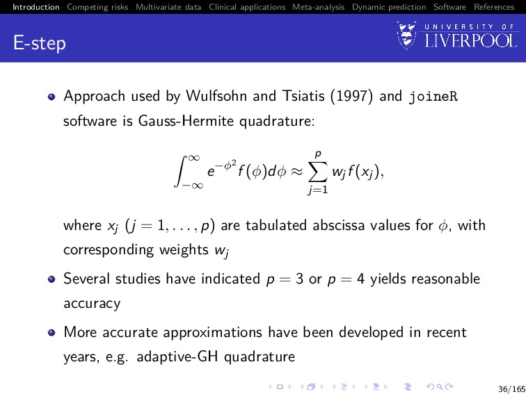
47. Introduction Competing risks Multivariate data Clinical applications Meta-analysis Dynamic prediction Software References E-step Approach used by Wulfsohn and Tsiatis (1997) and joineR software is Gauss-Hermite quadrature: ∞ −∞ e−φ2 f (φ)dφ ≈ p j=1 wjf (xj), where xj (j = 1, . . . , p) are tabulated abscissa values for φ, with corresponding weights wj Several studies have indicated p = 3 or p = 4 yields reasonable accuracy More accurate approximations have been developed in recent years, e.g. adaptive-GH quadrature 36/165
48. Introduction Competing risks Multivariate data Clinical applications Meta-analysis Dynamic prediction Software References Standard errors Hsieh et al. (2006) demonstrated that the profile likelihood approach in the EM algorithm leads to underestimation in the SEs, so recommended bootstrapping Conceptually simple: 1 sample n subjects with replacement and re-label with indices i = 1, . . . , n 2 re-fit the model to the bootstrap-sampled dataset 3 repeat steps 1 and 2 B-times, for each iteration extracting the model parameter estimates for (β , vech(D), σ2, γv , γy ) 4 calculate SEs of B sets of estimates Notice no SEs calculated for λ0(t), but that’s generally not of inferential interest 37/165
49. Introduction Competing risks Multivariate data Clinical applications Meta-analysis Dynamic prediction Software References Software We can implement all of this in the R package joineR with the general recipe: 1 Create a jointdata object using the joineR::jointdata() function 2 Fit a joint model using the joineR::joint() function 3 Calculate SEs using joineR::jointSE() function Each piece can be used in separate auxiliary functions along the way 38/165
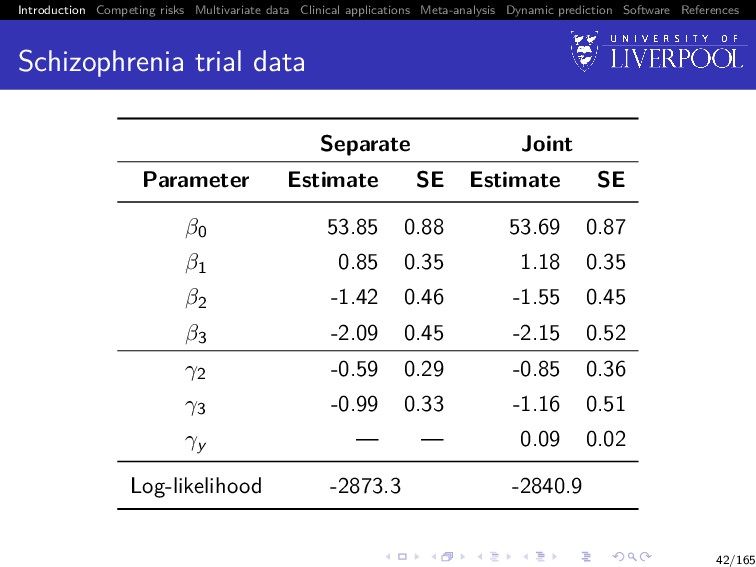
50. Introduction Competing risks Multivariate data Clinical applications Meta-analysis Dynamic prediction Software References Schizophrenia trial data Recall question from slide 16: Question Does the decrease in PANSS profiles reflects a genuine change over time or an artefact caused by selective dropout ⇒ Let’s fit a joint model between longitudinal PANSS score and time-to-dropout 39/165
51. Introduction Competing risks Multivariate data Clinical applications Meta-analysis Dynamic prediction Software References Schizophrenia trial data Longitudinal sub-model Yi (t) = β0 + β1t + 3 k=2 βkI(Xi = k)t + W1i (t) + εi (t) W1i (t) = bi0 + bi1t (bi0, bi1) ∼ N2(0, D) εi (t) i.i.d. ∼ N(0, σ2) Time-to-event sub-model λi (t) = λ0(t) exp 3 k=2 γkI(Xi = k) + W2i (t) W2i (t) = γy W1i (t) 40/165
52. Introduction Competing risks Multivariate data Clinical applications Meta-analysis Dynamic prediction Software References Example code # Set-up the data in a jointdata object data(mental) mental.unbalanced <- to.unbalanced(mental, id.col = 1, times = c(0, 1, 2, 4, 6, 8), Y.col = 2:7, other.col = 8:11) names(mental.unbalanced)[3] <- "Y" mental.long <- mental.unbalanced[, 1:3] mental.surv <- UniqueVariables(mental.unbalanced, 6:7, id.col = 1) mental.baseline <- UniqueVariables(mental.unbalanced, 4, id.col = 1) mental.jd <- jointdata( mental.long, mental.surv, mental.baseline, id.col = "id", time.col = "time") # Fit the joint model model.joint <- joint( mental.jd, Y ˜ time + time:treat, Surv(surv.time, cens.ind) ˜ treat, model = "intslope") # Bootstrap SEs model.jointSE <- jointSE(model.joint, 100) 41/165
53. Introduction Competing risks Multivariate data Clinical applications Meta-analysis Dynamic prediction Software References Schizophrenia trial data Separate Joint Parameter Estimate SE Estimate SE β0 53.85 0.88 53.69 0.87 β1 0.85 0.35 1.18 0.35 β2 -1.42 0.46 -1.55 0.45 β3 -2.09 0.45 -2.15 0.52 γ2 -0.59 0.29 -0.85 0.36 γ3 -0.99 0.33 -1.16 0.51 γy — — 0.09 0.02 Log-likelihood -2873.3 -2840.9 42/165
54. Introduction Competing risks Multivariate data Clinical applications Meta-analysis Dynamic prediction Software References Extension I: Competing risks events 43/165
55. Introduction Competing risks Multivariate data Clinical applications Meta-analysis Dynamic prediction Software References Motivation Joint models generally consider survival data that allows for one event with a single mode of failure and an assumption of independent censoring When there are several reasons why the failure event can occur, or some informative censoring occurs, it is known as competing risks 44/165
56. Introduction Competing risks Multivariate data Clinical applications Meta-analysis Dynamic prediction Software References SANAD trial data SANAD (Standard And New Antiepileptic Drugs) was a non-blinded randomized control trial recruiting patients with epilepsy to test anti-epilepsy drugs (AEDs) Patients were randomized to one of 5 antiepilepsy drugs (AEDs) Subgroup analysis (n = 605 patients) comparing 2 drugs: LTG (newer drug) vs. CBZ (standard) 45/165
57. Introduction Competing risks Multivariate data Clinical applications Meta-analysis Dynamic prediction Software References SANAD trial data Primary outcome was time to treatment failure, defined as the time to withdrawal of a randomised drug or addition of another/switch to an alternative AED Patients decided to switch to an alternative AED because of Inadequate seizure control (ISC; n = 94, 15%) Unacceptable adverse effects (UAE; n = 120, 20%) 46/165
58. Introduction Competing risks Multivariate data Clinical applications Meta-analysis Dynamic prediction Software References Clinical question Question Is LTG superior to CBZ in terms of (a) seizure control and (b) tolerability? 47/165
59. Introduction Competing risks Multivariate data Clinical applications Meta-analysis Dynamic prediction Software References Rationale for competing events Should we just analyse composite time-to-treatment failure for any reason? 48/165
60. Introduction Competing risks Multivariate data Clinical applications Meta-analysis Dynamic prediction Software References Rationale for competing events Should we just analyse composite time-to-treatment failure for any reason? No: assumes reasons of failure are of equal importance (which may not be the case): Loss of driving license due to continued seizures Side effects such as nausea, dizziness or rash 48/165
61. Introduction Competing risks Multivariate data Clinical applications Meta-analysis Dynamic prediction Software References Original results LTG is significantly more toler- able than CBZ 0.0 0.2 0.4 0.6 0.8 1.0 UAE Years Probability CBZ LTG 0 1 2 3 4 5 6 49/165
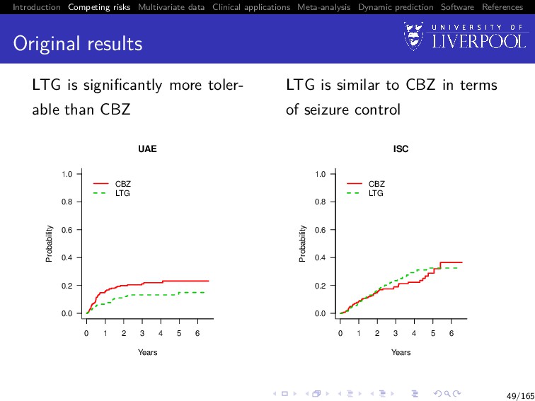
62. Introduction Competing risks Multivariate data Clinical applications Meta-analysis Dynamic prediction Software References Original results LTG is significantly more toler- able than CBZ 0.0 0.2 0.4 0.6 0.8 1.0 UAE Years Probability CBZ LTG 0 1 2 3 4 5 6 LTG is similar to CBZ in terms of seizure control 0.0 0.2 0.4 0.6 0.8 1.0 ISC Years Probability CBZ LTG 0 1 2 3 4 5 6 49/165
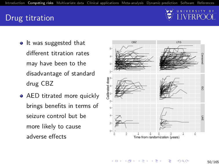
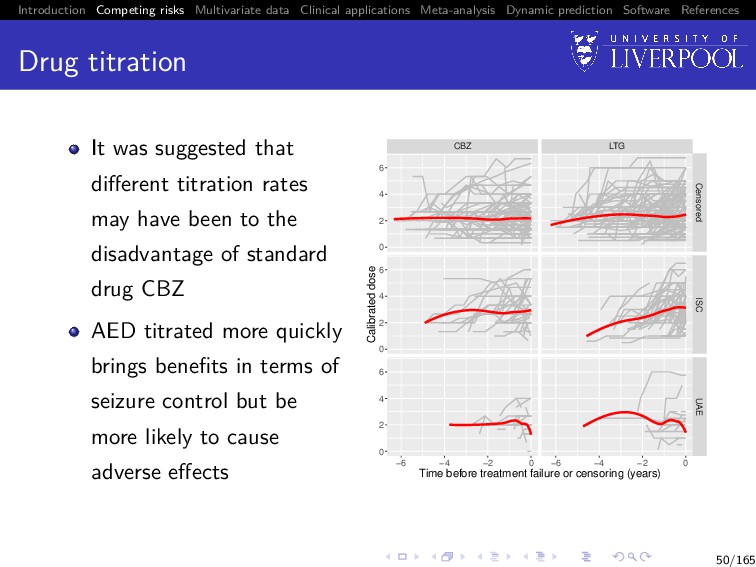
63. Introduction Competing risks Multivariate data Clinical applications Meta-analysis Dynamic prediction Software References Drug titration It was suggested that different titration rates may have been to the disadvantage of standard drug CBZ AED titrated more quickly brings benefits in terms of seizure control but be more likely to cause adverse effects CBZ LTG 0 2 4 6 0 2 4 6 0 2 4 6 Censored ISC UAE 0 2 4 6 0 2 4 6 Time from randomization (years) Calibrated dose 50/165
64. Introduction Competing risks Multivariate data Clinical applications Meta-analysis Dynamic prediction Software References Drug titration It was suggested that different titration rates may have been to the disadvantage of standard drug CBZ AED titrated more quickly brings benefits in terms of seizure control but be more likely to cause adverse effects CBZ LTG Censored ISC UAE −6 −4 −2 0 −6 −4 −2 0 0 2 4 6 0 2 4 6 0 2 4 6 Time before treatment failure or censoring (years) Calibrated dose 50/165
65. Introduction Competing risks Multivariate data Clinical applications Meta-analysis Dynamic prediction Software References Revised clinical questions Questions 1 Is drug titration associated with time to treatment failure for each cause? 2 After adjusting for drug titration is LTG still superior to CBZ in terms of UAE and ISC? 51/165
66. Introduction Competing risks Multivariate data Clinical applications Meta-analysis Dynamic prediction Software References Data For each subject i = 1, . . . , n, we observe An ni -vector of observed longitudinal measurements for the longitudinal outcome: yi = (yi1, . . . , yini ) Observation times tij for j = 1, . . . , ni , which can differ between subjects (Ti , δi ), where Ti = min(T∗ i , Ci ), where T∗ i is the true event time, Ci corresponds to a potential non-informative right-censoring time, and δi is the failure indicator equal to g (g = 1, . . . , G) if the failure is observed (T∗ i ≤ Ci ) and due to cause g, and 0 otherwise 52/165
67. Introduction Competing risks Multivariate data Clinical applications Meta-analysis Dynamic prediction Software References Model Longitudinal sub-model: same as for the univariate joint model Time-to-event sub-model: cause-specific hazards model 53/165
68. Introduction Competing risks Multivariate data Clinical applications Meta-analysis Dynamic prediction Software References Time-to-event sub-model Cause-specific hazards model with sub-model for cause g (g = 1, . . . , G): λ(g) i (t) = λ(g) 0 (t) exp vi γ(g) v + W (g) 2i (t) , where λ(g) 0 (·) (g = 1, . . . , G) are unspecified baseline hazard functions vi is a q-vector of baseline covariates with corresponding fixed effect terms γ(g) v (g = 1, . . . , G) W (g) 2i (t) (g = 1, . . . , G) are zero-mean latent Gaussian processes 54/165
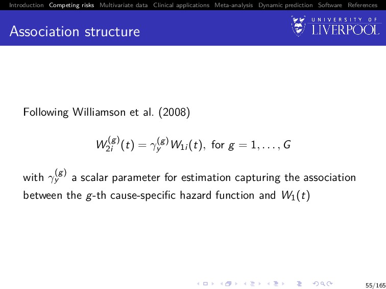
69. Introduction Competing risks Multivariate data Clinical applications Meta-analysis Dynamic prediction Software References Association structure Following Williamson et al. (2008) W (g) 2i (t) = γ(g) y W1i (t), for g = 1, . . . , G with γ(g) y a scalar parameter for estimation capturing the association between the g-th cause-specific hazard function and W1(t) 55/165
70. Introduction Competing risks Multivariate data Clinical applications Meta-analysis Dynamic prediction Software References Estimation & standard errors EM algorithm as per before, with exception that we now estimate G-pairs of λ(g) 0 (t), γ(g) y during the M-step Standard errors estimated using same bootstrap method 56/165
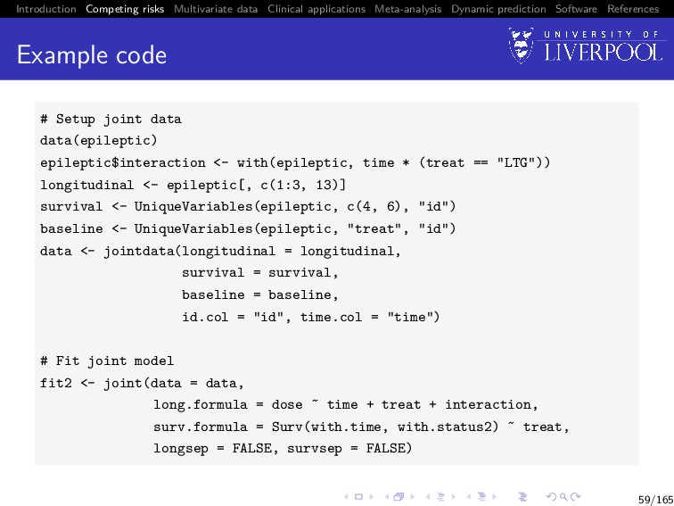
71. Introduction Competing risks Multivariate data Clinical applications Meta-analysis Dynamic prediction Software References Software We can fit these models in joineR using the same general work-flow as for the single failure type joint model joineR::joint() automatically detects presence of competing risks7 Currently limited to 2 failure types 7Requires failure types to be coded as 0 (censored), 1 (first failure type), 2 (second failure type). 57/165
72. Introduction Competing risks Multivariate data Clinical applications Meta-analysis Dynamic prediction Software References Epilepsy data Longitudinal sub-model: with Xi = 1 (LTG) vs. Xi = 0 (CBZ) Yi (t) = β0 + β1t + β2Xi + β3Xi × t + W1i (t) + εi (t) W1i = bi0 + bi1t (bi0, bi1) ∼ N2(0, D) εi (t) i.i.d. ∼ N(0, σ2) Time-to-event sub-model: with g ∈ {UAE, ISC} λ(g) i (t) = λ(g) 0 (t) exp γ(g) v Xi + W (g) 2i (t) W (g) 2i (t) = γ(g) y W1i (t) 58/165
73. Introduction Competing risks Multivariate data Clinical applications Meta-analysis Dynamic prediction Software References Example code # Setup joint data data(epileptic) epileptic$interaction <- with(epileptic, time * (treat == "LTG")) longitudinal <- epileptic[, c(1:3, 13)] survival <- UniqueVariables(epileptic, c(4, 6), "id") baseline <- UniqueVariables(epileptic, "treat", "id") data <- jointdata(longitudinal = longitudinal, survival = survival, baseline = baseline, id.col = "id", time.col = "time") # Fit joint model fit2 <- joint(data = data, long.formula = dose ˜ time + treat + interaction, surv.formula = Surv(with.time, with.status2) ˜ treat, longsep = FALSE, survsep = FALSE) 59/165
74. Introduction Competing risks Multivariate data Clinical applications Meta-analysis Dynamic prediction Software References Epilepsy data Est. SE 95% CI β0 (Intercept) 1.9730 0.0512 (1.8701, 2.0803) β1 time 0.0004 0.0001 (0.0002, 0.0005) β2 LTG -0.1381 0.0720 (-0.2908, -0.0307) β3 time × LTG 0.0006 0.0001 (0.0003, 0.0009) γ(UAE) v LTG -0.6602 0.2008 (-1.1063, -0.2338) γ(UAE) y Titration -0.9259 0.2600 (-1.4707, -0.4510) γ(ISC) v LTG 0.0272 0.1811 (-0.3940, 0.3306) γ(ISC) y Titration 0.5894 0.0873 (0.4031, 0.7513) 60/165
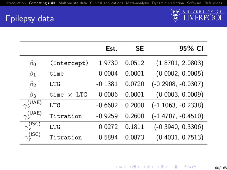
75. Introduction Competing risks Multivariate data Clinical applications Meta-analysis Dynamic prediction Software References Conclusion Is LTG superior to CBZ after adjusting for titration in terms of UAE? ISC? If LTG is titrated at the same rate as CBZ, the beneficial effect of LTG on UAE would still be evident LTG and CBZ still appear to provide similar seizure control 61/165
76. Introduction Competing risks Multivariate data Clinical applications Meta-analysis Dynamic prediction Software References Extension II: Multiple longitudinal outcomes 62/165
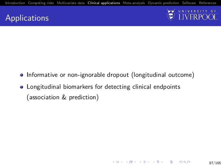
77. Introduction Competing risks Multivariate data Clinical applications Meta-analysis Dynamic prediction Software References Motivation Clinical studies often repeatedly measure multiple biomarkers or other measurements and an event time Research has predominantly focused on single measurement outcomes Harnessing all available information in a single model is advantageous and should lead to improved estimation and predictions 63/165
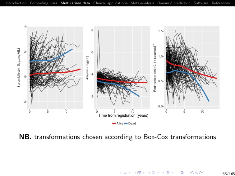
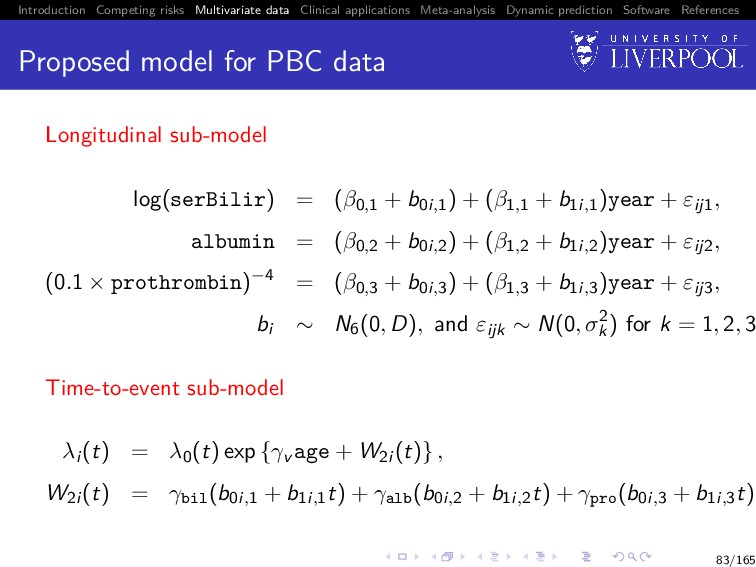
78. Introduction Competing risks Multivariate data Clinical applications Meta-analysis Dynamic prediction Software References The Mayo Clinic PBC data Primary biliary cirrhosis (PBC) is a chronic liver disease characterized by inflammatory destruction of the small bile ducts, which eventually leads to cirrhosis of the liver (Murtaugh et al. 1994) We analyse a subset of 154 patients randomized to placebo Multiple biomarkers repeatedly measured at intermittent times: 1 serum bilirubin (mg/dl) 2 serum albumin (mg/dl) 3 prothrombin time (seconds) Patients drop out if they die (ndie = 69, 44.8%) 64/165
79. Introduction Competing risks Multivariate data Clinical applications Meta-analysis Dynamic prediction Software References Prothrombin time (0.1 x seconds)−4 Albumin (mg dL) Serum bilirubin (loge mg dL) 0 5 10 0 5 10 0 5 10 0.0 0.5 1.0 1.5 2 4 6 8 −2 0 2 4 Time from registration (years) Alive Dead NB. transformations chosen according to Box-Cox transformations 65/165
80. Introduction Competing risks Multivariate data Clinical applications Meta-analysis Dynamic prediction Software References 0 2 4 6 8 10 12 14 0.0 0.2 0.4 0.6 0.8 1.0 Time from registration (years) Survival probability 66/165
81. Introduction Competing risks Multivariate data Clinical applications Meta-analysis Dynamic prediction Software References What is the state of the field? A large number of models published over recent years incorporating different outcome types; distributions, multivariate event times; estimation approaches; association structures; disease areas; etc. Early adoption into clinical literature, but a lack of software! 67/165
82. Introduction Competing risks Multivariate data Clinical applications Meta-analysis Dynamic prediction Software References Data For each subject i = 1, . . . , n, we observe yi = (yi1 , . . . , yiK ) is the K-variate continuous outcome vector, where each yik denotes an (nik × 1)-vector of observed longitudinal measurements for the k-th outcome type: yik = (yi1k, . . . , yinik k) Observation times tijk for j = 1, . . . , nik, which can differ between subjects and outcomes (Ti , δi ), where Ti = min(T∗ i , Ci ), where T∗ i is the true event time, Ci corresponds to a potential right-censoring time, and δi is the failure indicator equal to 1 if the failure is observed (T∗ i ≤ Ci ) and 0 otherwise 68/165
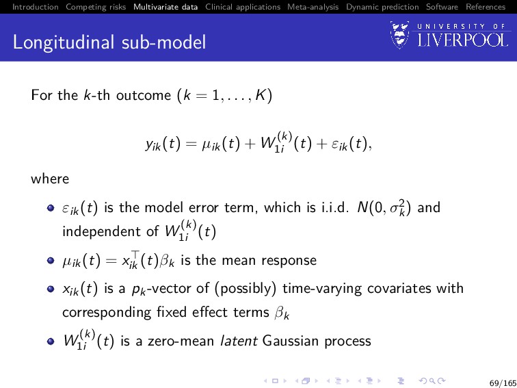
83. Introduction Competing risks Multivariate data Clinical applications Meta-analysis Dynamic prediction Software References Longitudinal sub-model For the k-th outcome (k = 1, . . . , K) yik(t) = µik(t) + W (k) 1i (t) + εik(t), where εik(t) is the model error term, which is i.i.d. N(0, σ2 k ) and independent of W (k) 1i (t) µik(t) = xik (t)βk is the mean response xik(t) is a pk-vector of (possibly) time-varying covariates with corresponding fixed effect terms βk W (k) 1i (t) is a zero-mean latent Gaussian process 69/165
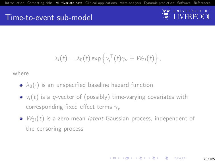
84. Introduction Competing risks Multivariate data Clinical applications Meta-analysis Dynamic prediction Software References Time-to-event sub-model λi (t) = λ0(t) exp vi (t)γv + W2i (t) , where λ0(·) is an unspecified baseline hazard function vi (t) is a q-vector of (possibly) time-varying covariates with corresponding fixed effect terms γv W2i (t) is a zero-mean latent Gaussian process, independent of the censoring process 70/165
85. Introduction Competing risks Multivariate data Clinical applications Meta-analysis Dynamic prediction Software References Association structure Extending Laird and Ware (1982) to the multivariate case: W (k) 1i (t) = zik (t)bik 71/165
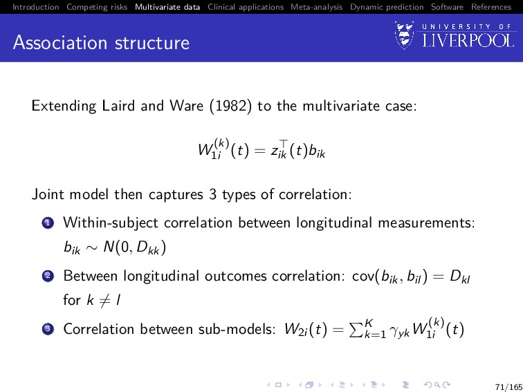
86. Introduction Competing risks Multivariate data Clinical applications Meta-analysis Dynamic prediction Software References Association structure Extending Laird and Ware (1982) to the multivariate case: W (k) 1i (t) = zik (t)bik Joint model then captures 3 types of correlation: 1 Within-subject correlation between longitudinal measurements: bik ∼ N(0, Dkk) 2 Between longitudinal outcomes correlation: cov(bik, bil ) = Dkl for k = l 3 Correlation between sub-models: W2i (t) = K k=1 γykW (k) 1i (t) 71/165
87. Introduction Competing risks Multivariate data Clinical applications Meta-analysis Dynamic prediction Software References Likelihood We can re-write the longitudinal sub-model as yi | bi , β, Σi ∼ N(Xi β + Zi bi , Σi ), with bi | D ∼ N(0, D), where β = (β1 , . . . , βK ), bi = (bi1 , . . . , biK ) , and Xi =      Xi1 · · · 0 . . . ... . . . 0 · · · XiK      , Zi =      Zi1 · · · 0 . . . ... . . . 0 · · · ZiK      , D =      D11 · · · D1K . . . ... . . . D1K · · · DKK      Σi =      σ2 1 Ini1 · · · 0 . . . ... . . . 0 · · · σ2 K IniK      72/165
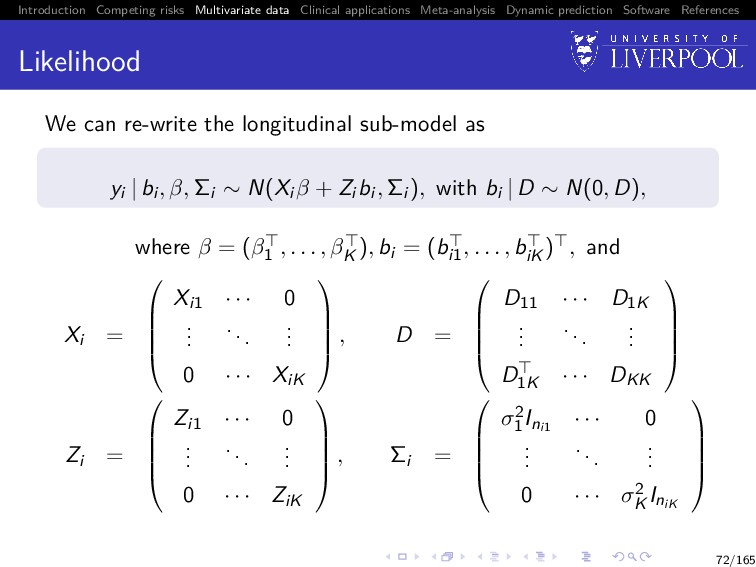
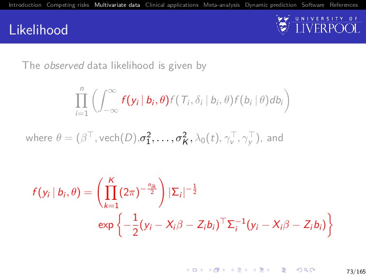
88. Introduction Competing risks Multivariate data Clinical applications Meta-analysis Dynamic prediction Software References Likelihood The observed data likelihood is given by n i=1 ∞ −∞ f (yi | bi , θ)f (Ti , δi | bi , θ)f (bi | θ)dbi where θ = (β , vech(D),σ2 1 , . . . , σ2 K , λ0(t), γv , γy ) 73/165
89. Introduction Competing risks Multivariate data Clinical applications Meta-analysis Dynamic prediction Software References Likelihood The observed data likelihood is given by n i=1 ∞ −∞ f (yi | bi , θ)f (Ti , δi | bi , θ)f (bi | θ)dbi where θ = (β , vech(D),σ2 1 , . . . , σ2 K , λ0(t), γv , γy ), and f (yi | bi , θ) = K k=1 (2π)−nik 2 |Σi |−1 2 exp − 1 2 (yi − Xi β − Zi bi ) Σ−1 i (yi − Xi β − Zi bi ) 73/165
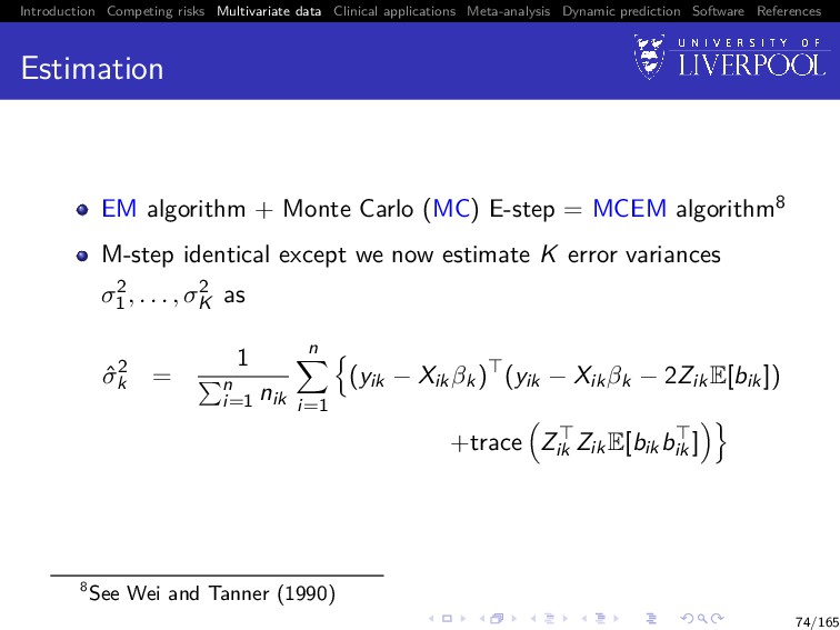
90. Introduction Competing risks Multivariate data Clinical applications Meta-analysis Dynamic prediction Software References Estimation EM algorithm + Monte Carlo (MC) E-step = MCEM algorithm8 M-step identical except we now estimate K error variances σ2 1 , . . . , σ2 K as ˆ σ2 k = 1 n i=1 nik n i=1 (yik − Xikβk) (yik − Xikβk − 2ZikE[bik]) +trace Zik ZikE[bikbik ] 8See Wei and Tanner (1990) 74/165
91. Introduction Competing risks Multivariate data Clinical applications Meta-analysis Dynamic prediction Software References E-step E h(bi ) | Ti , δi , yi ; ˆ θ = ∞ −∞ h(bi )f (bi | yi ; ˆ θ)f (Ti , δi | bi ; ˆ θ)dbi ∞ −∞ f (bi | yi ; ˆ θ)f (Ti , δi | bi ; ˆ θ)dbi , where h(·) = any known fuction, bi | yi , θ ∼ N Ai Zi Σ−1 i (yi − Xi β) , Ai , and Ai = Zi Σ−1 i Zi + D−1 −1 75/165
92. Introduction Competing risks Multivariate data Clinical applications Meta-analysis Dynamic prediction Software References Monte Carlo E-step Replace the Gauss-Hermite quadrature with a Monte Carlo approximation for scalability with increasing K and/or dim(bi ) E h(bi ) | Ti , δi , yi ; ˆ θ = ∞ −∞ h(bi )f (bi | yi ; ˆ θ)f (Ti , δi | bi ; ˆ θ)dbi ∞ −∞ f (bi | yi ; ˆ θ)f (Ti , δi | bi ; ˆ θ)dbi , 76/165
93. Introduction Competing risks Multivariate data Clinical applications Meta-analysis Dynamic prediction Software References Monte Carlo E-step Replace the Gauss-Hermite quadrature with a Monte Carlo approximation for scalability with increasing K and/or dim(bi ) E h(bi ) | Ti , δi , yi ; ˆ θ ≈ 1 N N d=1 h b(d) i f Ti , δi | b(d) i ; ˆ θ 1 N N d=1 f Ti , δi | b(d) i ; ˆ θ where b(1) i , b(2) i , . . . , b(N) i are a random sample from bi | yi , θ 76/165
94. Introduction Competing risks Multivariate data Clinical applications Meta-analysis Dynamic prediction Software References Monte Carlo E-step As proposed by Henderson et al. (2000), we use antithetic simulation for variance reduction instead of directly sampling from the MVN distribution for bi | yi ; ˆ θ: Sample Ω ∼ N(0, Ir ) and obtain the pairs Ai Zi Σ−1 i (yi − Xi β) ± Ci Ω, where Ci is the Cholesky decomposition of Ai such that Ci Ci = Ai Negative correlation between the pairs ⇒ smaller variance in the sample means than would be obtained from N independent simulations 77/165
95. Introduction Competing risks Multivariate data Clinical applications Meta-analysis Dynamic prediction Software References Convergence In standard EM, convergence usually declared at (m + 1)-th iteration if one of the following criteria satisfied 1 Relative change: ∆(m+1) rel = max |ˆ θ(m+1)−ˆ θ(m)| |ˆ θ(m)|+ 1 < 0 2 Absolute change: ∆(m+1) abs = max |ˆ θ(m+1) − ˆ θ(m)| < 2 for some choice of 0, 1, and 2 Note: joineR uses criterion #2 78/165
96. Introduction Competing risks Multivariate data Clinical applications Meta-analysis Dynamic prediction Software References Convergence In MCEM framework, there are 2 complications to account for 79/165
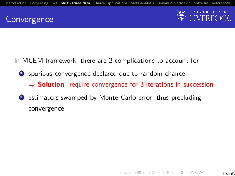
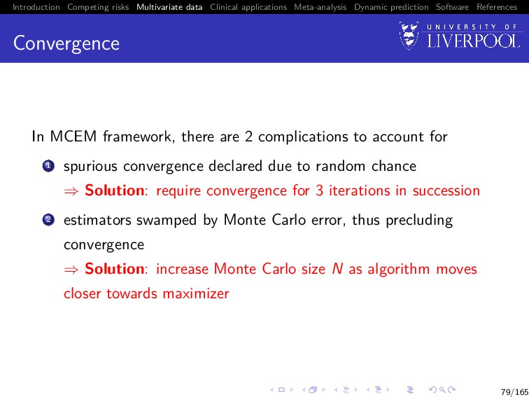
97. Introduction Competing risks Multivariate data Clinical applications Meta-analysis Dynamic prediction Software References Convergence In MCEM framework, there are 2 complications to account for 1 spurious convergence declared due to random chance 79/165
98. Introduction Competing risks Multivariate data Clinical applications Meta-analysis Dynamic prediction Software References Convergence In MCEM framework, there are 2 complications to account for 1 spurious convergence declared due to random chance ⇒ Solution: require convergence for 3 iterations in succession 79/165
99. Introduction Competing risks Multivariate data Clinical applications Meta-analysis Dynamic prediction Software References Convergence In MCEM framework, there are 2 complications to account for 1 spurious convergence declared due to random chance ⇒ Solution: require convergence for 3 iterations in succession 2 estimators swamped by Monte Carlo error, thus precluding convergence 79/165
100. Introduction Competing risks Multivariate data Clinical applications Meta-analysis Dynamic prediction Software References Convergence In MCEM framework, there are 2 complications to account for 1 spurious convergence declared due to random chance ⇒ Solution: require convergence for 3 iterations in succession 2 estimators swamped by Monte Carlo error, thus precluding convergence ⇒ Solution: increase Monte Carlo size N as algorithm moves closer towards maximizer 79/165
101. Introduction Competing risks Multivariate data Clinical applications Meta-analysis Dynamic prediction Software References Convergence Using large N when far from maximizer = computationally inefficient Using small N when close to maximizer = unlikely to detect convergence Solution (proposed by Ripatti et al. 2002): after a ‘burn-in’ phase, calculate the coefficient of variation statistic cv(∆(m+1) rel ) = sd(∆(m−1) rel , ∆(m) rel , ∆(m+1) rel ) mean(∆(m−1) rel , ∆(m) rel , ∆(m+1) rel ) , and increase N to N + N/δ if cv(∆(m+1) rel ) > cv(∆(m) rel ) for some small positive integer δ 80/165
102. Introduction Competing risks Multivariate data Clinical applications Meta-analysis Dynamic prediction Software References Standard error estimation We could use bootstrap method again, but it is getting slow as dim(θ) increases Instead, we approximate the information matrix of θ−λ0(t) (with λ0(t) profiled out of the likelihood) by the empirical information matrix (McLachlan and Krishnan 2008): Ie(θ) = n i=1 si (θ)si (θ) − 1 n S(θ)S (θ), S(θ) = n i=1 si (θ) is the score vector Then use SE(θ) ≈ I−1/2 e (ˆ θ) 81/165
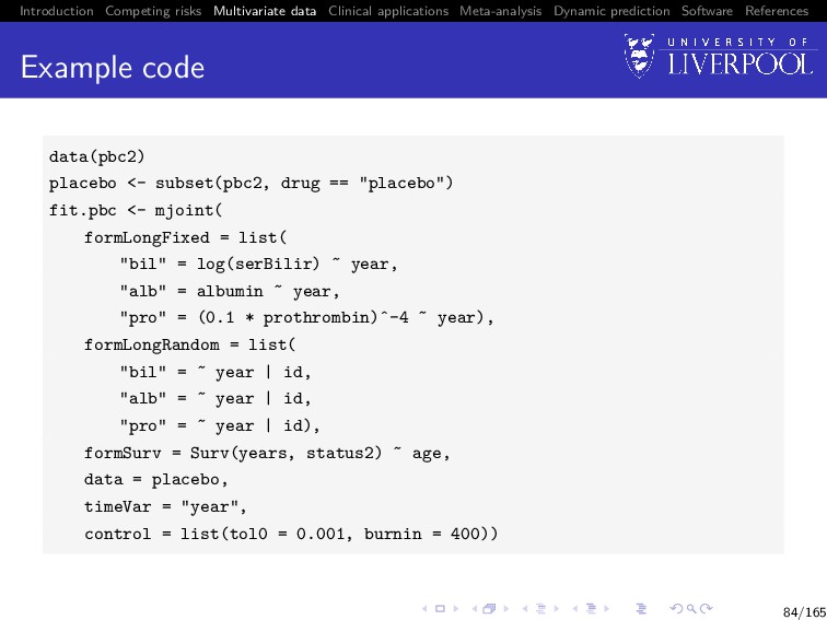
103. Introduction Competing risks Multivariate data Clinical applications Meta-analysis Dynamic prediction Software References Software We can implement all of this in the R package joineRML Single function required: joineRML::mjoint() Package can also be used to fit univariate joint models, but using MCEM rather than EM optimisation Calculates approximate SEs by default, but bootstrap SEs available via joineRML::bootSE() 82/165
104. Introduction Competing risks Multivariate data Clinical applications Meta-analysis Dynamic prediction Software References Proposed model for PBC data Longitudinal sub-model log(serBilir) = (β0,1 + b0i,1) + (β1,1 + b1i,1)year + εij1, albumin = (β0,2 + b0i,2) + (β1,2 + b1i,2)year + εij2, (0.1 × prothrombin)−4 = (β0,3 + b0i,3) + (β1,3 + b1i,3)year + εij3, bi ∼ N6(0, D), and εijk ∼ N(0, σ2 k ) for k = 1, 2, 3 Time-to-event sub-model λi (t) = λ0(t) exp {γv age + W2i (t)} , W2i (t) = γbil (b0i,1 + b1i,1t) + γalb (b0i,2 + b1i,2t) + γpro (b0i,3 + b1i,3t). 83/165
105. Introduction Competing risks Multivariate data Clinical applications Meta-analysis Dynamic prediction Software References Example code data(pbc2) placebo <- subset(pbc2, drug == "placebo") fit.pbc <- mjoint( formLongFixed = list( "bil" = log(serBilir) ˜ year, "alb" = albumin ˜ year, "pro" = (0.1 * prothrombin)ˆ-4 ˜ year), formLongRandom = list( "bil" = ˜ year | id, "alb" = ˜ year | id, "pro" = ˜ year | id), formSurv = Surv(years, status2) ˜ age, data = placebo, timeVar = "year", control = list(tol0 = 0.001, burnin = 400)) 84/165
106. Introduction Competing risks Multivariate data Clinical applications Meta-analysis Dynamic prediction Software References Results Parameter Estimate SE 95% CI β0,1 0.5541 0.0858 (0.3859, 0.7223) β1,1 0.2009 0.0201 (0.1616, 0.2402) β0,2 3.5549 0.0356 (3.4850, 3.6248) β1,2 -0.1245 0.0101 (-0.1444, -0.1047) β0,3 0.8304 0.0212 (0.7888, 0.8719) β1,3 -0.0577 0.0062 (-0.0699, -0.0456) γv 0.0462 0.0151 (0.0166, 0.0759) γbil 0.8181 0.2046 (0.4171, 1.2191) γalb -1.7060 0.6181 (-2.9173, -0.4946) γpro -2.2085 1.6070 (-5.3582, 0.9412) 85/165
107. Introduction Competing risks Multivariate data Clinical applications Meta-analysis Dynamic prediction Software References Applications in clinical research 86/165
108. Introduction Competing risks Multivariate data Clinical applications Meta-analysis Dynamic prediction Software References Applications Informative or non-ignorable dropout (longitudinal outcome) Longitudinal biomarkers for detecting clinical endpoints (association & prediction) 87/165
109. Introduction Competing risks Multivariate data Clinical applications Meta-analysis Dynamic prediction Software References Magnetic The largest, randomised, double-blind, placebo-controlled study to-date in acute severe asthma in children 88/165
110. Introduction Competing risks Multivariate data Clinical applications Meta-analysis Dynamic prediction Software References Magnetic Objective: Determine whether the use of nebulised MgSO4, when given as an adjunct to standard therapy for 60 minutes results in a clinical improvement compared with standard treatment alone Enrolled children from 30 hospitals in the UK with acute severe asthma who did not respond to standard inhaled treatment Design: Randomly allocated (1:1) to receive the standard nebuliser with isotonic MgSO4 or placebo (isotonic saline) on three occasions at 20 minutes intervals 252 children were randomised to the magnesium group and 256 to the placebo group 89/165
111. Introduction Competing risks Multivariate data Clinical applications Meta-analysis Dynamic prediction Software References The question Clinical question Does the addition of nebulised MgSO4 to the standard nebulised treatment significantly effect the clinical outcome of an Asthma Severity Scores (ASS) at 60 minutes post treatment? 90/165
112. Introduction Competing risks Multivariate data Clinical applications Meta-analysis Dynamic prediction Software References ASS (Asthma Severity Score) Three components, each scored as 0, 1, 2, 3 ASS ranges from 0 (best) to 9 (worst) Assessments were completed at baseline, 20, 40, 60, 120, 180 and 240 minutes post randomisation Primary endpoint: ASS at 60 minutes post-randomisation Secondary question: Is any observed effect sustained following end of treatment at 60 minutes? 91/165
113. Introduction Competing risks Multivariate data Clinical applications Meta-analysis Dynamic prediction Software References Primary outcome results The mean difference in ASS at T60 between the two treatment groups, magnesium minus placebo, adjusting for baseline ASS, was -0.25 points (95% CI -0.48 to -0.02 points), i.e. magnesium appears to lower the score 92/165
114. Introduction Competing risks Multivariate data Clinical applications Meta-analysis Dynamic prediction Software References 93/165
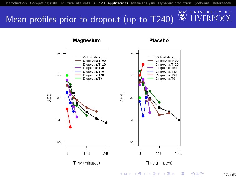
115. Introduction Competing risks Multivariate data Clinical applications Meta-analysis Dynamic prediction Software References Why joint modelling? To address the problem of non-ignorable missing ASS data The joint model combines the information from the dropout pattern and variations in ASS over time The mean profiles are almost identical for both magnesium and placebo groups However, this pattern could be an artefact of selective drop out, and it would be a biased comparison between treatment groups unless it is adjusted with joint modelling 94/165
116. Introduction Competing risks Multivariate data Clinical applications Meta-analysis Dynamic prediction Software References Mean profiles prior to dropout (up to T60) Shows that dropout in magnesium group occurred because patients get better (most children were clinically well and ready to discharge) whilst dropout in placebo occurred is because patients get worse 95/165
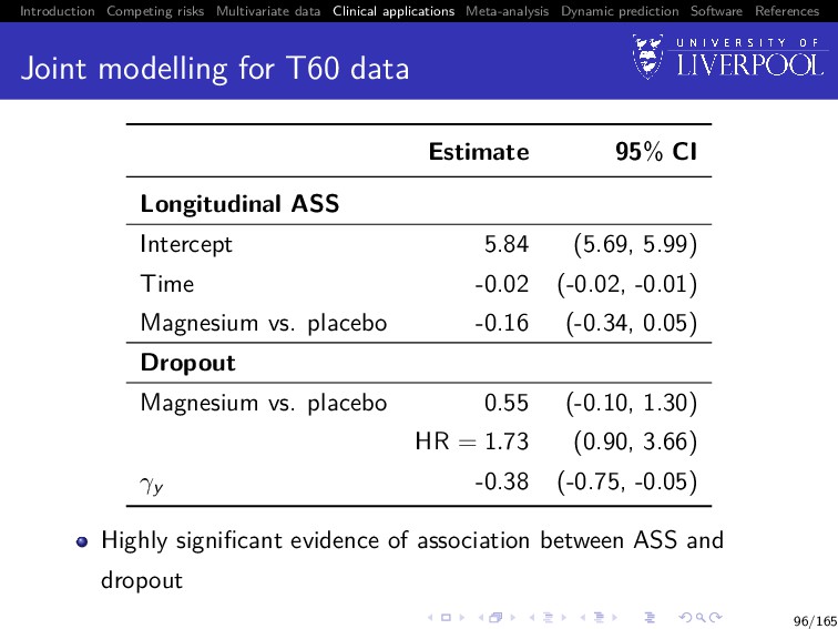
117. Introduction Competing risks Multivariate data Clinical applications Meta-analysis Dynamic prediction Software References Joint modelling for T60 data Estimate 95% CI Longitudinal ASS Intercept 5.84 (5.69, 5.99) Time -0.02 (-0.02, -0.01) Magnesium vs. placebo -0.16 (-0.34, 0.05) Dropout Magnesium vs. placebo 0.55 (-0.10, 1.30) HR = 1.73 (0.90, 3.66) γy -0.38 (-0.75, -0.05) Highly significant evidence of association between ASS and dropout 96/165
118. Introduction Competing risks Multivariate data Clinical applications Meta-analysis Dynamic prediction Software References Mean profiles prior to dropout (up to T240) 97/165
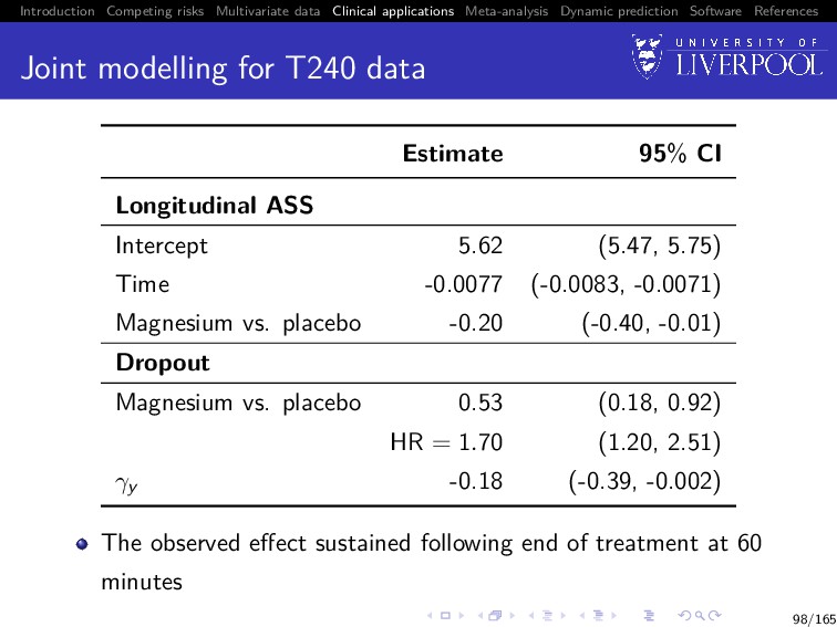
119. Introduction Competing risks Multivariate data Clinical applications Meta-analysis Dynamic prediction Software References Joint modelling for T240 data Estimate 95% CI Longitudinal ASS Intercept 5.62 (5.47, 5.75) Time -0.0077 (-0.0083, -0.0071) Magnesium vs. placebo -0.20 (-0.40, -0.01) Dropout Magnesium vs. placebo 0.53 (0.18, 0.92) HR = 1.70 (1.20, 2.51) γy -0.18 (-0.39, -0.002) The observed effect sustained following end of treatment at 60 minutes 98/165
120. Introduction Competing risks Multivariate data Clinical applications Meta-analysis Dynamic prediction Software References TIPIT A randomised controlled trial of thyroxine in preterm infants under 28 weeks’ gestation 99/165
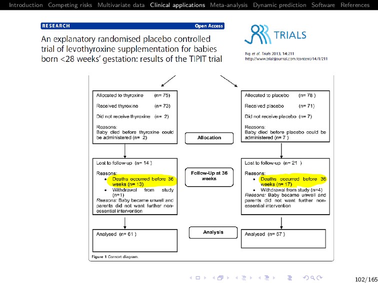
121. Introduction Competing risks Multivariate data Clinical applications Meta-analysis Dynamic prediction Software References TIPIT Infants born at extreme prematurity (below 28 weeks’ gestation) are at high risk of developmental disability A major risk factor for disability is having a low level of thyroid hormone which is recognised to be a frequent phenomenon in these infants It is unclear whether low levels of thyroid hormone are a cause of disability, or a consequence of concurrent adversity In this explanatory multicentre double blind randomised placebo controlled trial, 153 infants born below 28 weeks gestation were randomised to levothyroxine (LT4) supplementation or placebo until 32 weeks corrected gestational age 100/165
122. Introduction Competing risks Multivariate data Clinical applications Meta-analysis Dynamic prediction Software References The question Clinical question How treatment with levothyroxine postnatally until 32 weeks corrected gestational age (CGA) modulates brain size and development? The free T4 fraction (FT4) is a measure of how the thyroid is functioning FT4 measured at 0, 14, 21, 28 and 36 weeks post-randomisation 101/165
123. Introduction Competing risks Multivariate data Clinical applications Meta-analysis Dynamic prediction Software References 102/165
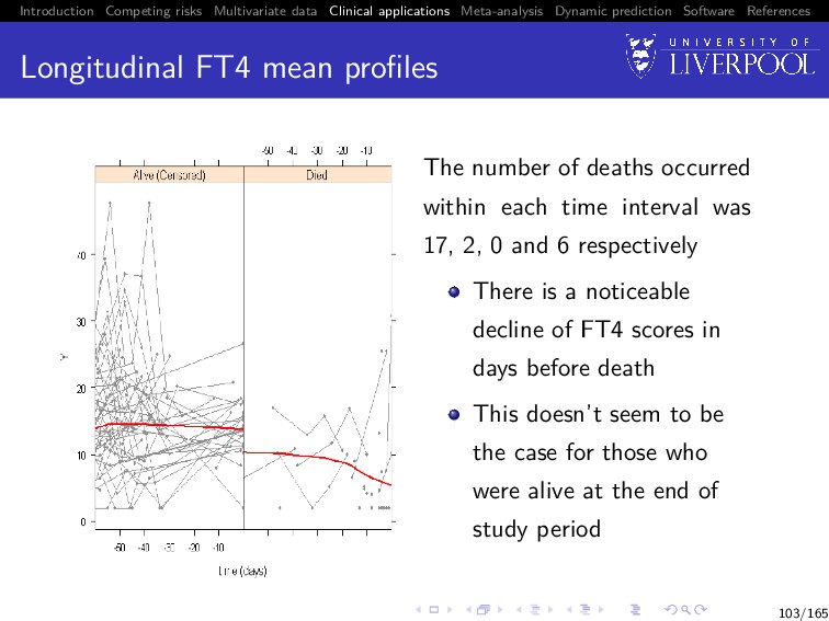
124. Introduction Competing risks Multivariate data Clinical applications Meta-analysis Dynamic prediction Software References Longitudinal FT4 mean profiles The number of deaths occurred within each time interval was 17, 2, 0 and 6 respectively There is a noticeable decline of FT4 scores in days before death This doesn’t seem to be the case for those who were alive at the end of study period 103/165
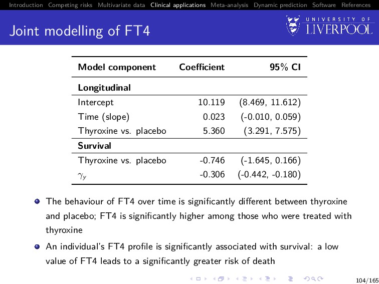
125. Introduction Competing risks Multivariate data Clinical applications Meta-analysis Dynamic prediction Software References Joint modelling of FT4 Model component Coefficient 95% CI Longitudinal Intercept 10.119 (8.469, 11.612) Time (slope) 0.023 (-0.010, 0.059) Thyroxine vs. placebo 5.360 (3.291, 7.575) Survival Thyroxine vs. placebo -0.746 (-1.645, 0.166) γy -0.306 (-0.442, -0.180) The behaviour of FT4 over time is significantly different between thyroxine and placebo; FT4 is significantly higher among those who were treated with thyroxine An individual’s FT4 profile is significantly associated with survival: a low value of FT4 leads to a significantly greater risk of death 104/165
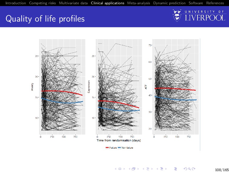
126. Introduction Competing risks Multivariate data Clinical applications Meta-analysis Dynamic prediction Software References SANAD: Quality of life Increasingly recognised as an important outcome in epilepsy - concern about worsening over time Postal assessments sent out at baseline, 3 months, 1 year, 2 year Typical QoL data structure – infrequent, variable response times Measures chosen to represent the emotional, social and physical effects of AEDs and epilepsy: Adverse events profile (problems in past 4 weeks): tiredness, headaches, rash, sleepiness, etc. Anxiety score (past week) Depression score (past week) 105/165
127. Introduction Competing risks Multivariate data Clinical applications Meta-analysis Dynamic prediction Software References The question Clinical question Does poor QoL lead to the failure of initial choice of treatment? 106/165
128. Introduction Competing risks Multivariate data Clinical applications Meta-analysis Dynamic prediction Software References Analysis A subgroup of 486 patients randomised to CBZ and LTG 176 (36.2%) had failed initial treatment 1313 records of QoL in total 107/165
129. Introduction Competing risks Multivariate data Clinical applications Meta-analysis Dynamic prediction Software References Quality of life profiles 108/165
130. Introduction Competing risks Multivariate data Clinical applications Meta-analysis Dynamic prediction Software References Results for the association QoL Association 95% CI P Anxiety -0.0055 (-0.1041, 0.0930) 0.9121 Depression 0.0002 (-0.0901, 0.0905) 0.9968 AEP 0.0451 (0.0011, 0.0891) 0.0446 109/165
131. Introduction Competing risks Multivariate data Clinical applications Meta-analysis Dynamic prediction Software References Does poor QoL lead to treatment failure? No statistical evidence that anxiety or depression are associated with the failure of initial treatment Continued high score on adverse events profile leads failure of the initial treatment 110/165
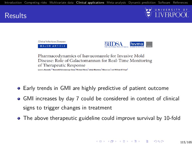
132. Introduction Competing risks Multivariate data Clinical applications Meta-analysis Dynamic prediction Software References SECURE trial A phase 3, randomized, double-blind study comparing Isavuconazole (new drug) versus Voriconazole (standard drug) in patients with invasive aspergillosis (IA) IA is a persistent public health problem Therapeutic options are few and limited by toxicity The evaluation of the use of galactomannan (GM) as a biomarker for diagnosing IA was pre-specified as a secondary objective 111/165
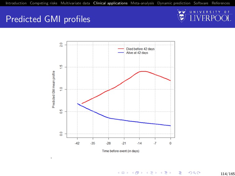
133. Introduction Competing risks Multivariate data Clinical applications Meta-analysis Dynamic prediction Software References The question Clinical question Identify an early pattern of GM index (GMI) that could guide therapeutic decision-making for patients with IA 112/165
134. Introduction Competing risks Multivariate data Clinical applications Meta-analysis Dynamic prediction Software References Joint model to address Intermittently measured GMI measurements Missingness in daily measurement schedule over 42 days Leads to misleading inference about the true association between a prospective biomarker and subsequent risk of clinical endpoint Measurement error (laboratory error + errors induced during specimen collection & storage) hinders the explanatory power of the biomarker causing the estimated parameters to be biased towards the null 113/165
135. Introduction Competing risks Multivariate data Clinical applications Meta-analysis Dynamic prediction Software References Predicted GMI profiles 114/165
136. Introduction Competing risks Multivariate data Clinical applications Meta-analysis Dynamic prediction Software References Results Early trends in GMI are highly predictive of patient outcome GMI increases by day 7 could be considered in context of clinical signs to trigger changes in treatment The above therapeutic guideline could improve survival by 10-fold 115/165
137. Introduction Competing risks Multivariate data Clinical applications Meta-analysis Dynamic prediction Software References Extension III: Meta-analysis 116/165
138. Introduction Competing risks Multivariate data Clinical applications Meta-analysis Dynamic prediction Software References Current application of joint models 6 5 4 3 2 1 0 5 10 15 20 1997 1998 1999 2000 2001 2002 2003 2004 2005 2006 2007 2008 2009 2010 2011 2012 2013 2014 2015 Year of Publication Count Indentified study by Year of Publication 117/165
139. Introduction Competing risks Multivariate data Clinical applications Meta-analysis Dynamic prediction Software References Basic joint model specification Longitudinal Ykij = g (W1kij (t), θ1 ) + εkij Ykij = X1kij β1k + Z(2) kij b(2) ki + εkij Association W2ki (t) = f (W1ki ) Time-to-Event λki (t) = λ0 (t) exp {h(W2ki (t), θ2 )} λki (t) = λ0 (t) exp {X2ki β2k + W2ki (t)} 118/165
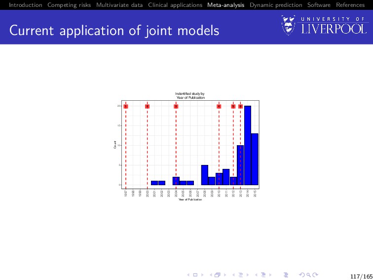
140. Introduction Competing risks Multivariate data Clinical applications Meta-analysis Dynamic prediction Software References What is meta-analysis (MA)? Systematic pooling of results from multiple studies Allows for: increased precision identification of effect sizes too small to be identified in single studies questions additional to those originally posed in the data to be answered 119/165
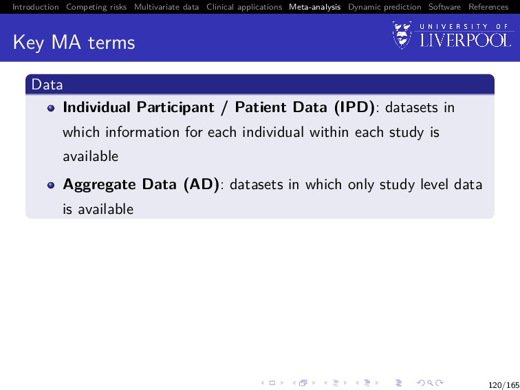
141. Introduction Competing risks Multivariate data Clinical applications Meta-analysis Dynamic prediction Software References Key MA terms Data Individual Participant / Patient Data (IPD): datasets in which information for each individual within each study is available Aggregate Data (AD): datasets in which only study level data is available 120/165
142. Introduction Competing risks Multivariate data Clinical applications Meta-analysis Dynamic prediction Software References Key MA terms Data Individual Participant / Patient Data (IPD): datasets in which information for each individual within each study is available Aggregate Data (AD): datasets in which only study level data is available Stage Two-stage MA: meta-analyses where models are fitted to the data from each study, and the study specific parameters pooled using standard meta-analytic techniques One-Stage MA: meta-analyses where data from all studies in held in a large meta-dataset, and a single model fitted 120/165
143. Introduction Competing risks Multivariate data Clinical applications Meta-analysis Dynamic prediction Software References Two-Stage MA of joint data Process: 1 Preliminaries: decide on most appropriate modelling structure 2 First stage: fit joint models to data from each included study, and extract parameters of interest 3 Second stage: pool parameters using standard meta-analytic techniques 121/165
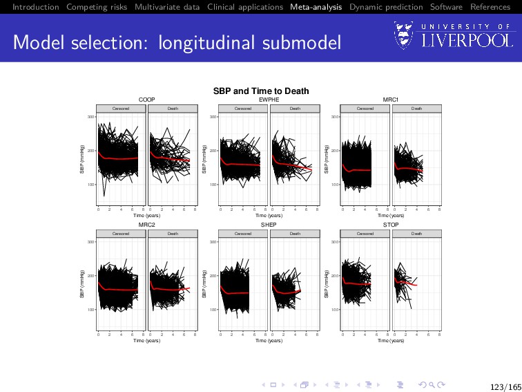
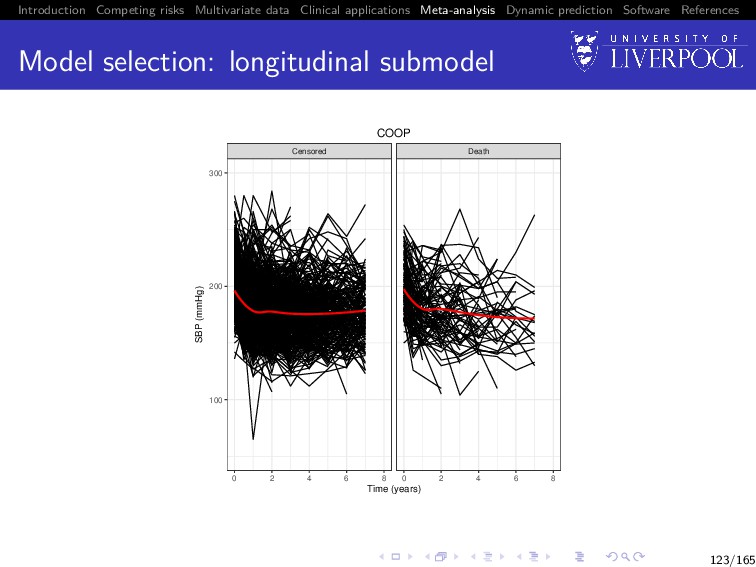
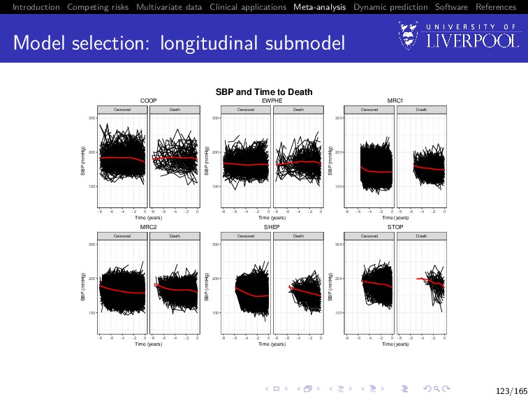
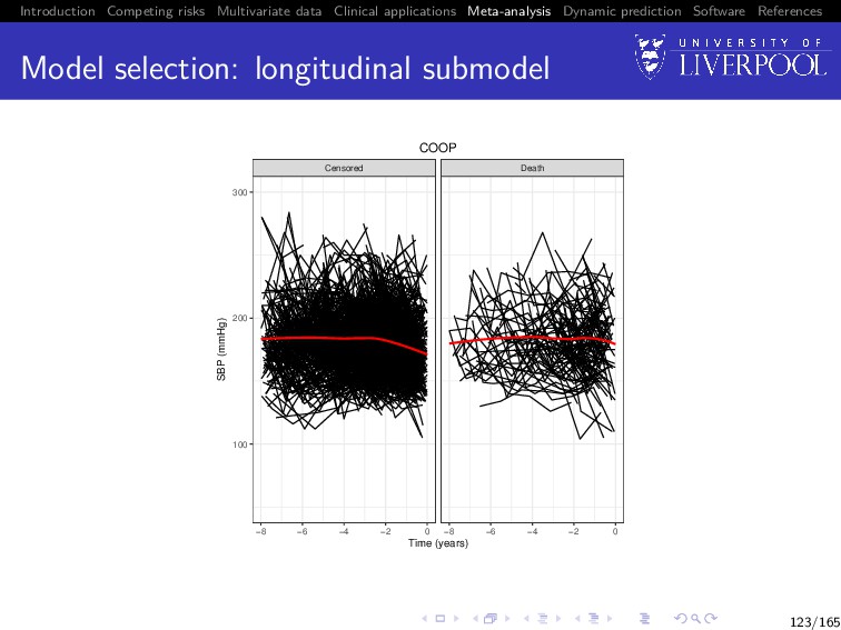
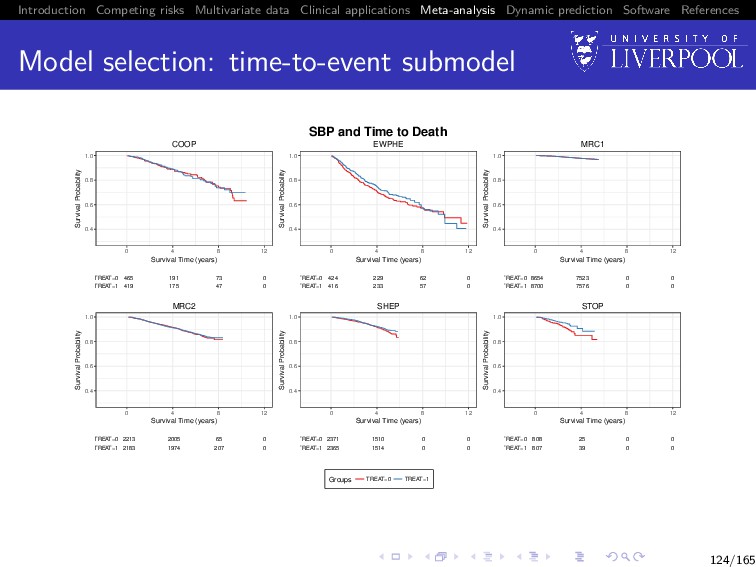
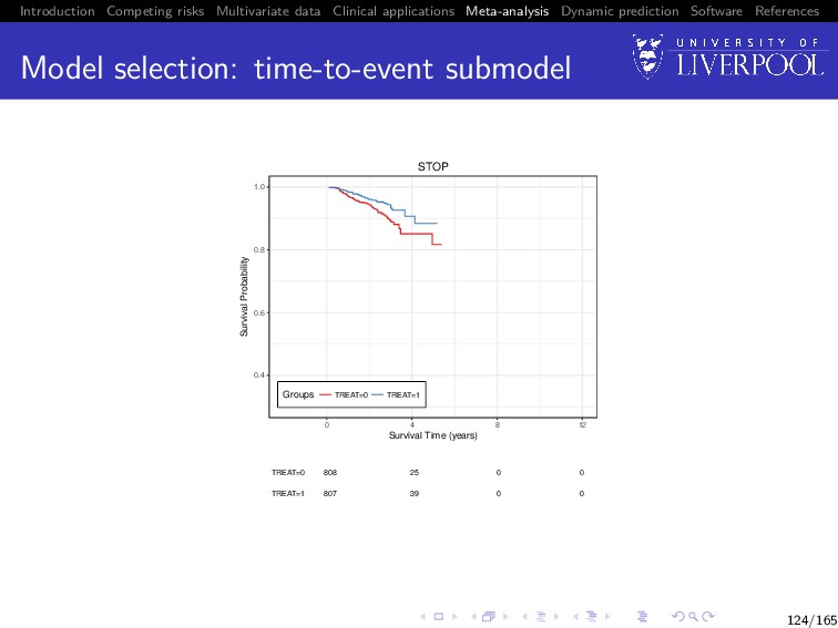
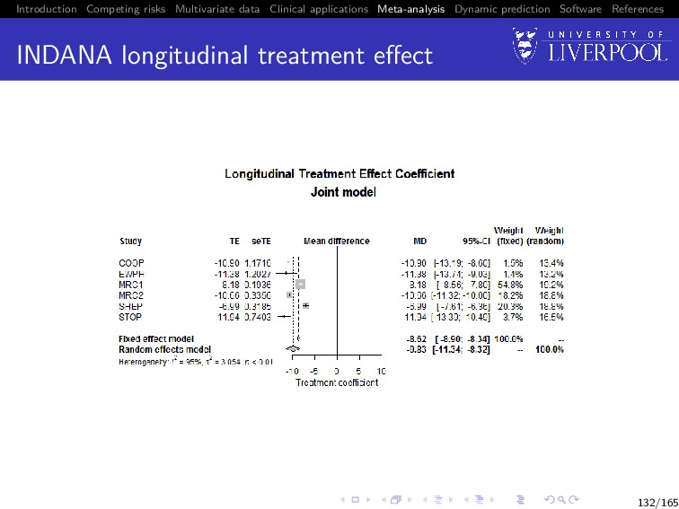
144. Introduction Competing risks Multivariate data Clinical applications Meta-analysis Dynamic prediction Software References Clinical example The process of a two stage MA using joint data will be demonstrated using a subset of the INDANA dataset (Gueyffier 1995, Sudell et al. 2017) Multi-study dataset of hypertensive patients containing studies COOP, EWPHE, MRC1, MRC2, SHEP, STOP Examples model longitudinal systolic blood pressure (SBP) and time until death 122/165
145. Introduction Competing risks Multivariate data Clinical applications Meta-analysis Dynamic prediction Software References Model selection: longitudinal submodel Censored Death 0 2 4 6 8 0 2 4 6 8 100 200 300 Time (years) SBP (mmHg) COOP Censored Death 0 2 4 6 8 0 2 4 6 8 100 200 300 Time (years) SBP (mmHg) EWPHE Censored Death 0 2 4 6 8 0 2 4 6 8 100 200 300 Time (years) SBP (mmHg) MRC1 Censored Death 0 2 4 6 8 0 2 4 6 8 100 200 300 Time (years) SBP (mmHg) MRC2 Censored Death 0 2 4 6 8 0 2 4 6 8 100 200 300 Time (years) SBP (mmHg) SHEP Censored Death 0 2 4 6 8 0 2 4 6 8 100 200 300 Time (years) SBP (mmHg) STOP SBP and Time to Death 123/165
146. Introduction Competing risks Multivariate data Clinical applications Meta-analysis Dynamic prediction Software References Model selection: longitudinal submodel Censored Death 0 2 4 6 8 0 2 4 6 8 100 200 300 Time (years) SBP (mmHg) COOP 123/165
147. Introduction Competing risks Multivariate data Clinical applications Meta-analysis Dynamic prediction Software References Model selection: longitudinal submodel Censored Death −8 −6 −4 −2 0 −8 −6 −4 −2 0 100 200 300 Time (years) SBP (mmHg) COOP Censored Death −8 −6 −4 −2 0 −8 −6 −4 −2 0 100 200 300 Time (years) SBP (mmHg) EWPHE Censored Death −8 −6 −4 −2 0 −8 −6 −4 −2 0 100 200 300 Time (years) SBP (mmHg) MRC1 Censored Death −8 −6 −4 −2 0 −8 −6 −4 −2 0 100 200 300 Time (years) SBP (mmHg) MRC2 Censored Death −8 −6 −4 −2 0 −8 −6 −4 −2 0 100 200 300 Time (years) SBP (mmHg) SHEP Censored Death −8 −6 −4 −2 0 −8 −6 −4 −2 0 100 200 300 Time (years) SBP (mmHg) STOP SBP and Time to Death 123/165
148. Introduction Competing risks Multivariate data Clinical applications Meta-analysis Dynamic prediction Software References Model selection: longitudinal submodel Censored Death −8 −6 −4 −2 0 −8 −6 −4 −2 0 100 200 300 Time (years) SBP (mmHg) COOP 123/165
149. Introduction Competing risks Multivariate data Clinical applications Meta-analysis Dynamic prediction Software References Model selection: time-to-event submodel TREAT=0 465 191 73 0 TREAT=1 419 175 47 0 0.4 0.6 0.8 1.0 0 4 8 12 Survival Time (years) Survival Probability COOP TREAT=0 424 229 62 0 TREAT=1 416 233 57 0 0.4 0.6 0.8 1.0 0 4 8 12 Survival Time (years) Survival Probability EWPHE TREAT=0 8654 7523 0 0 TREAT=1 8700 7576 0 0 0.4 0.6 0.8 1.0 0 4 8 12 Survival Time (years) Survival Probability MRC1 TREAT=0 2213 2005 65 0 TREAT=1 2183 1974 207 0 0.4 0.6 0.8 1.0 0 4 8 12 Survival Time (years) Survival Probability MRC2 TREAT=0 2371 1510 0 0 TREAT=1 2365 1514 0 0 0.4 0.6 0.8 1.0 0 4 8 12 Survival Time (years) Survival Probability SHEP TREAT=0 808 25 0 0 TREAT=1 807 39 0 0 0.4 0.6 0.8 1.0 0 4 8 12 Survival Time (years) Survival Probability STOP Groups TREAT=0 TREAT=1 SBP and Time to Death 124/165
150. Introduction Competing risks Multivariate data Clinical applications Meta-analysis Dynamic prediction Software References Model selection: time-to-event submodel TREAT=0 808 25 0 0 TREAT=1 807 39 0 0 0.4 0.6 0.8 1.0 0 4 8 12 Survival Time (years) Survival Probability Groups TREAT=0 TREAT=1 STOP 124/165
151. Introduction Competing risks Multivariate data Clinical applications Meta-analysis Dynamic prediction Software References Model selection: association structure The association structure should be selected based on the clinical background of the data Example 1 Scenario: clinicians believe that individuals with blood pressure recorded above the population average at a given time point are at higher risk of death 125/165
152. Introduction Competing risks Multivariate data Clinical applications Meta-analysis Dynamic prediction Software References Model selection: association structure The association structure should be selected based on the clinical background of the data Example 1 Scenario: clinicians believe that individuals with blood pressure recorded above the population average at a given time point are at higher risk of death Answer 1 Random effects only association structure W2ki (t) = γk Z(2) ki b(2) ki 125/165
153. Introduction Competing risks Multivariate data Clinical applications Meta-analysis Dynamic prediction Software References Model selection: association structure The association structure should be selected based on the clinical background of the data Example 2 Scenario: clinicians believe the higher the recorded blood pressure for an individual at a given time point, the higher their risk of death 125/165
154. Introduction Competing risks Multivariate data Clinical applications Meta-analysis Dynamic prediction Software References Model selection: association structure The association structure should be selected based on the clinical background of the data Example 2 Scenario: clinicians believe the higher the recorded blood pressure for an individual at a given time point, the higher their risk of death Answer 2 Current value association structure: W2ki (t) = γk X1ki β1k + Z(2) ki b(2) ki 125/165
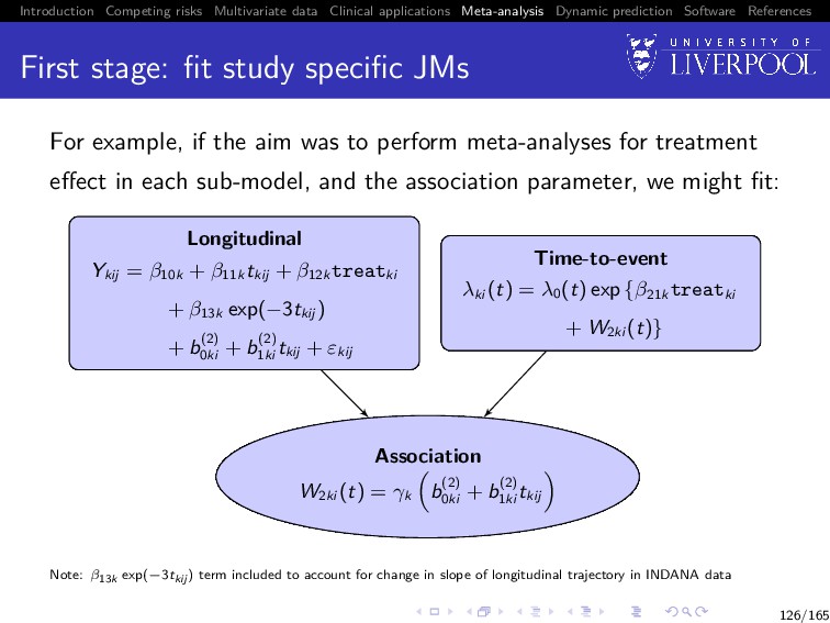
155. Introduction Competing risks Multivariate data Clinical applications Meta-analysis Dynamic prediction Software References First stage: fit study specific JMs For example, if the aim was to perform meta-analyses for treatment effect in each sub-model, and the association parameter, we might fit: Longitudinal Ykij = β10k + β11k tkij + β12k treatki + β13k exp(−3tkij ) + b(2) 0ki + b(2) 1ki tkij + εkij Association W2ki (t) = γk b(2) 0ki + b(2) 1ki tkij Time-to-event λki (t) = λ0 (t) exp {β21k treatki + W2ki (t)} Note: β13k exp(−3tkij ) term included to account for change in slope of longitudinal trajectory in INDANA data 126/165
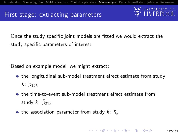
156. Introduction Competing risks Multivariate data Clinical applications Meta-analysis Dynamic prediction Software References First stage: extracting parameters Once the study specific joint models are fitted we would extract the study specific parameters of interest Based on example model, we might extract: the longitudinal sub-model treatment effect estimate from study k: ˆ β12k the time-to-event sub-model treatment effect estimate from study k: ˆ β21k the association parameter from study k: ˆ γk 127/165
157. Introduction Competing risks Multivariate data Clinical applications Meta-analysis Dynamic prediction Software References Second stage: pooling results We then pool the study specific parameters (e.g. ˆ β12k) using inverse variance approach to obtain an overall pooled estimate (e.g. ˆ β12) using: ˆ β12 = K k=1 wk ˆ β12k K k=1 wk 128/165
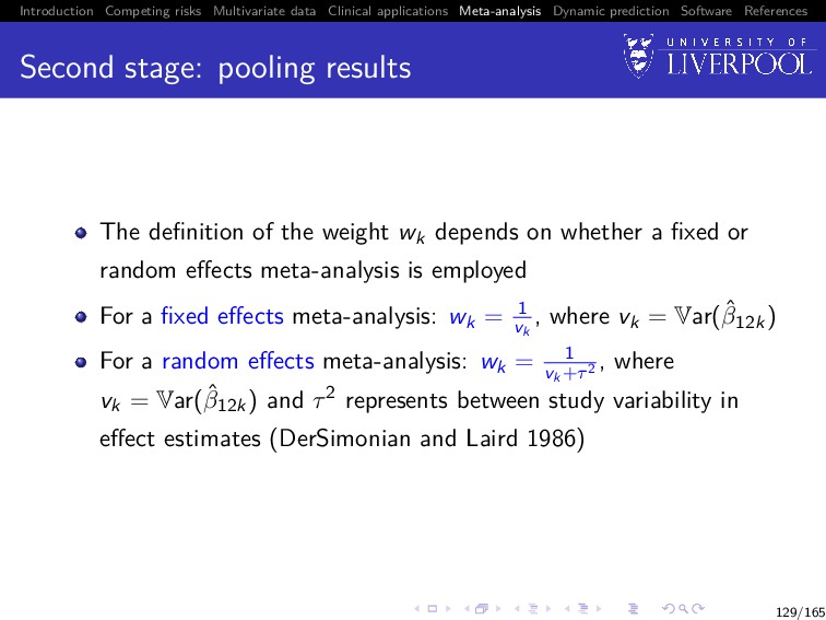
158. Introduction Competing risks Multivariate data Clinical applications Meta-analysis Dynamic prediction Software References Second stage: pooling results The definition of the weight wk depends on whether a fixed or random effects meta-analysis is employed For a fixed effects meta-analysis: wk = 1 vk , where vk = Var(ˆ β12k) For a random effects meta-analysis: wk = 1 vk +τ2 , where vk = Var(ˆ β12k) and τ2 represents between study variability in effect estimates (DerSimonian and Laird 1986) 129/165
159. Introduction Competing risks Multivariate data Clinical applications Meta-analysis Dynamic prediction Software References Fixed effect or random effect approach? Fixed effect approaches: assume the true parameter is constant across all studies any variation between study specific parameter estimates can be attributed to measurement error do not account for possible heterogeneity between studies 130/165
160. Introduction Competing risks Multivariate data Clinical applications Meta-analysis Dynamic prediction Software References Fixed effect or random effect approach? Random effect approaches: assume the study specific parameter estimates are realizations from a common random variable treats included studies as a random sample from eligible studies, but meta-analysis aims to include all eligible studies, so use of random MA is debated accounts for possible heterogeneity between studies might assign more weight to smaller studies than a fixed MA in the presence of heterogeneity (potentially invalid assumption) Note: if there is no between study heterogeneity in your dataset, the fixed and random effects approaches should give the same result 131/165
161. Introduction Competing risks Multivariate data Clinical applications Meta-analysis Dynamic prediction Software References INDANA longitudinal treatment effect 132/165
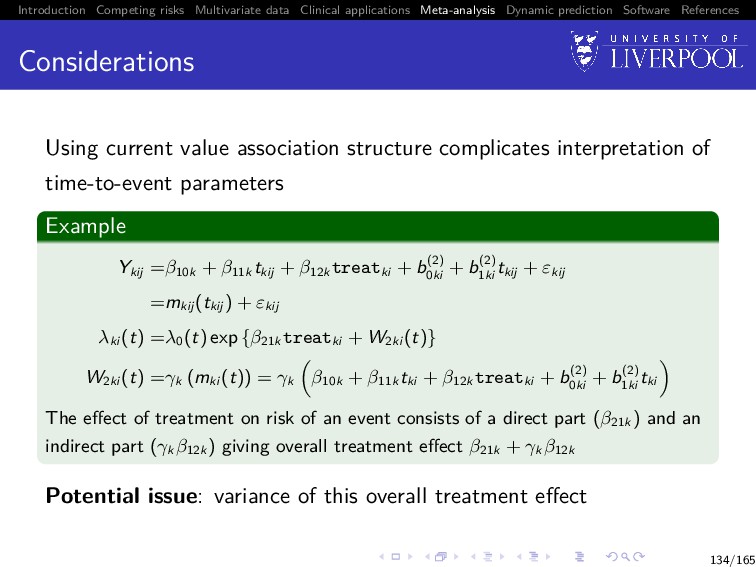
162. Introduction Competing risks Multivariate data Clinical applications Meta-analysis Dynamic prediction Software References Considerations The interpretation of the association parameter depends on the specification of the joint model Example 1: different association structures Joint model 1 uses a proportional random effect only association structure: W2ki (t) = γk Z(2) ki b(2) ki Joint model 2 uses a current value association structure: W2ki (t) = γk X1ki β1 + Z(2) ki b(2) ki 133/165
163. Introduction Competing risks Multivariate data Clinical applications Meta-analysis Dynamic prediction Software References Considerations The interpretation of the association parameter depends on the specification of the joint model Example 2: same association structure, different sub-model specification Both joint model fits use a proportional random effect only association structure Joint model 1 involves only a random intercept: W2ki (t) = γk(Z(2) ki b(2) ki ) = γk(b(2) 0ki ) Joint model 2 involves both a random intercept and random slope: W2ki (t) = γk(Z(2) ki b(2) ki ) = γk(b(2) 0ki + b(2) 1ki tki ) 133/165
164. Introduction Competing risks Multivariate data Clinical applications Meta-analysis Dynamic prediction Software References Considerations Using current value association structure complicates interpretation of time-to-event parameters Example Ykij =β10k + β11k tkij + β12k treatki + b(2) 0ki + b(2) 1ki tkij + εkij =mkij (tkij ) + εkij λki (t) =λ0 (t) exp {β21k treatki + W2ki (t)} W2ki (t) =γk (mki (t)) = γk β10k + β11k tki + β12k treatki + b(2) 0ki + b(2) 1ki tki The effect of treatment on risk of an event consists of a direct part (β21k ) and an indirect part (γk β12k ) giving overall treatment effect β21k + γk β12k Potential issue: variance of this overall treatment effect 134/165
165. Introduction Competing risks Multivariate data Clinical applications Meta-analysis Dynamic prediction Software References Two-Stage MA process overview Preliminaries: Produce plots of longitudinal trajectories panelled by event type Produce Kaplan-Meier plots of the time-to-event outcome Use plots to determine appropriate sub-model structures Determine most appropriate association structure (with reference to clinical background) 135/165
166. Introduction Competing risks Multivariate data Clinical applications Meta-analysis Dynamic prediction Software References Two-Stage MA process overview First Stage: Group studies such that the chosen model structure in each group is identical Within each group fit identical sub-models to data from each study Extract estimates of parameters of interest from study specific joint model fits, along with standard errors 136/165
167. Introduction Competing risks Multivariate data Clinical applications Meta-analysis Dynamic prediction Software References Two-Stage MA process overview Second Stage: Pool estimates within each group using standard meta-analytic techniques Results between groups should be qualitatively compared through discussion, but not quantitatively pooled 137/165
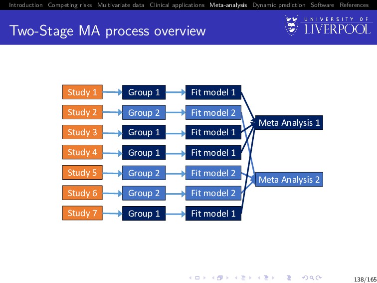
168. Introduction Competing risks Multivariate data Clinical applications Meta-analysis Dynamic prediction Software References Two-Stage MA process overview Study 1 Study 2 Study 3 Study 6 Study 4 Study 5 Study 7 Group 1 Group 2 Group 1 Group 2 Group 2 Group 1 Group 1 Fit model 1 Fit model 2 Fit model 1 Fit model 2 Fit model 2 Fit model 1 Fit model 1 Meta Analysis 1 Meta Analysis 2 138/165
169. Introduction Competing risks Multivariate data Clinical applications Meta-analysis Dynamic prediction Software References One-Stage MA of Joint Data Two-stage methods Automatically account for clustering of data within studies One-stage methods Have to account for membership of individuals within studies in some way Methods include: fixed study membership term, and interactions between study membership and other parameters study level random effects stratification of baseline hazard by study in time-to-event sub-model 139/165
170. Introduction Competing risks Multivariate data Clinical applications Meta-analysis Dynamic prediction Software References Software The joineRmeta package contains functions for: Producing study specific plots of longitudinal and time-to-event data Easily performing the second stage of two stage MA of joint data Fitting one-stage multi-level joint meta-analytic models Optional practical question on this after lunch 140/165
171. Introduction Competing risks Multivariate data Clinical applications Meta-analysis Dynamic prediction Software References Extension IV: Dynamic prediction 141/165
172. Introduction Competing risks Multivariate data Clinical applications Meta-analysis Dynamic prediction Software References Dynamic prediction So far we have only discussed inference from joint models Dynamic prediction Can we predict: 1 failure probability at time u > t given longitudinal data observed up until time t 2 Longitudinal trajectories at time u > t given longitudinal data observed up until time t Utility of multivariate data Do we gain from using multiple longitudinal outcomes? 142/165
173. Introduction Competing risks Multivariate data Clinical applications Meta-analysis Dynamic prediction Software References Dynamic prediction: survival For a new subject i = n + 1 with available longitudinal measurements yn+1{t} up to time t, we want to calculate P[T∗ n+1 ≥ u | T∗ n+1 > t, yn+1{t}; θ] = E Sn+1 (u | bn+1; θ) Sn+1 (t | bn+1; θ) , where the expectation is taken with respect to the distribution p(bn+1 | T∗ n+1 > t, yn+1{t}; θ), and Sn+1 (u | bn+1; θ) = exp − u 0 λ0(s) exp{vn+1 (s)γv + Wn+1(s)}ds 143/165
174. Introduction Competing risks Multivariate data Clinical applications Meta-analysis Dynamic prediction Software References Dynamic prediction: survival Rizopoulos (2011) proposed two estimators for this: 1. First-order approximation P[T∗ n+1 ≥ u | T∗ n+1 > t, yn+1{t}; θ] ≈ Sn+1 u | ˆ bn+1 ; ˆ θ Sn+1 t | ˆ bn+1 ; ˆ θ , where ˆ bn+1 is the mode of p(bn+1 | T∗ n+1 > t, yn+1{t}; ˆ θ) 2. Simulated scheme 1 Draw θ(l) ∼ N(ˆ θ, V (ˆ θ)) 2 Draw b(l) n+1 ∼ p(bn+1 | T∗ n+1 > t, yn+1{t}; θ(l)) [Metropolis-Hastings] 3 Calculate Sn+1 u | b(l) n+1 ;θ(l) Sn+1 t | b(l) n+1 ;θ(l) 4 Repeat Steps 1–3 for l = 2, . . . , L 144/165
175. Introduction Competing risks Multivariate data Clinical applications Meta-analysis Dynamic prediction Software References Example code # New patient nd <- subset(placebo, id == "11") # patient 11 # First-order prediction (default) pred1 <- dynSurv(fit.pbc, nd[1:5, ]) pred1 plot(pred1) # Simulated prediction pred2 <- dynSurv(fit.pbc, nd[1:5, ], type = "simulated", scale = 2) pred2 plot(pred2) 145/165
176. Introduction Competing risks Multivariate data Clinical applications Meta-analysis Dynamic prediction Software References Example code First order approximation 0.2 0.3 0.4 0.5 0.6 0.7 0.8 data.t$tk[[k]] log, serBilir 3.7 3.8 3.9 4.0 4.1 data.t$tk[[k]] albumin 0.45 0.50 0.55 0.60 0.65 data.t$tk[[k]] ^, (0.1 * prothrombin), −4 0 2 4 6 8 10 12 14 xpts ypts 0.0 0.2 0.4 0.6 0.8 1.0 Time Event−free probability 146/165
177. Introduction Competing risks Multivariate data Clinical applications Meta-analysis Dynamic prediction Software References Example code Simulated scheme 0.2 0.3 0.4 0.5 0.6 0.7 0.8 data.t$tk[[k]] log, serBilir 3.7 3.8 3.9 4.0 4.1 data.t$tk[[k]] albumin 0.45 0.50 0.55 0.60 0.65 data.t$tk[[k]] ^, (0.1 * prothrombin), −4 0 2 4 6 8 10 12 14 xpts ypts 0.0 0.2 0.4 0.6 0.8 1.0 Time Event−free probability 146/165
178. Introduction Competing risks Multivariate data Clinical applications Meta-analysis Dynamic prediction Software References Example code Simulated scheme + constrained B-spline smoother 0.2 0.3 0.4 0.5 0.6 0.7 0.8 data.t$tk[[k]] log, serBilir 3.7 3.8 3.9 4.0 4.1 data.t$tk[[k]] albumin 0.45 0.50 0.55 0.60 0.65 data.t$tk[[k]] ^, (0.1 * prothrombin), −4 0 2 4 6 8 10 12 14 xpts ypts 0.0 0.2 0.4 0.6 0.8 1.0 Time Event−free probability 146/165
179. Introduction Competing risks Multivariate data Clinical applications Meta-analysis Dynamic prediction Software References Truly dynamic prediction 147/165 0.20 0.25 0.30 0.35 0.40 0.45 data.t$tk[[k]] log, serBilir 2.5 3.0 3.5 4.0 4.5 5.0 5.5 data.t$tk[[k]] albumin 0.3 0.4 0.5 0.6 data.t$tk[[k]] ^, (0.1 * prothrombin), −4 0 0 2 4 6 8 10 12 14 xpts ypts 0.0 0.2 0.4 0.6 0.8 1.0 Time Event−free probability
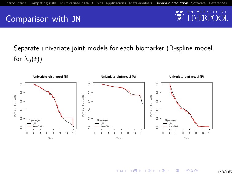
180. Introduction Competing risks Multivariate data Clinical applications Meta-analysis Dynamic prediction Software References Comparison with JM Separate univariate joint models for each biomarker (B-spline model for λ0(t)) 0 2 4 6 8 10 12 14 0.0 0.2 0.4 0.6 0.8 1.0 Univariate joint model {B} Time Pr(Ti ≥ u | Ti > t, y ~ i (t)) R package JM joineRML 0 2 4 6 8 10 12 14 0.0 0.2 0.4 0.6 0.8 1.0 Univariate joint model {A} Time Pr(Ti ≥ u | Ti > t, y ~ i (t)) R package JM joineRML 0 2 4 6 8 10 12 14 0.0 0.2 0.4 0.6 0.8 1.0 Univariate joint model {P} Time Pr(Ti ≥ u | Ti > t, y ~ i (t)) R package JM joineRML 148/165
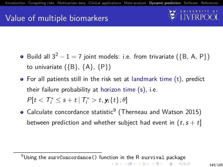
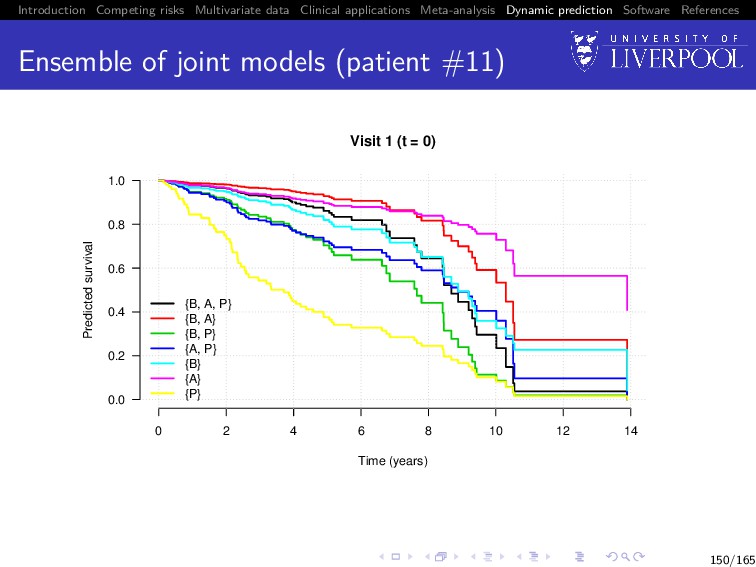
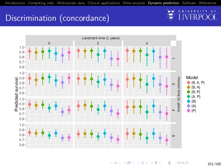
181. Introduction Competing risks Multivariate data Clinical applications Meta-analysis Dynamic prediction Software References Value of multiple biomarkers Build all 32 − 1 = 7 joint models: i.e. from trivariate ({B, A, P}) to univariate ({B}, {A}, {P}) For all patients still in the risk set at landmark time (t), predict their failure probability at horizon time (s), i.e. P[t < T∗ i ≤ s + t | T∗ i > t, yi {t}; θ] Calculate concordance statistic9 (Therneau and Watson 2015) between prediction and whether subject had event in (t, s + t] 9Using the survConcordance() function in the R survival package 149/165
182. Introduction Competing risks Multivariate data Clinical applications Meta-analysis Dynamic prediction Software References Ensemble of joint models (patient #11) 150/165 0 2 4 6 8 10 12 14 0.0 0.2 0.4 0.6 0.8 1.0 Visit 1 (t = 0) Time (years) Predicted survival {B, A, P} {B, A} {B, P} {A, P} {B} {A} {P}
183. Introduction Competing risks Multivariate data Clinical applications Meta-analysis Dynamic prediction Software References Discrimination (concordance) q q q q q q q q q q q q q q q q q q q q q q q q q q q q q q q q q q q q q q q q q q q q q q q q q q q q q q q q q q q q q q q q q q q q q q q q q q q q q q q q q q q q 0 2 4 1 2 4 8 Landmark time (t; years) Horizon time (s; years) 0.6 0.7 0.8 0.9 1.0 0.6 0.7 0.8 0.9 1.0 0.6 0.7 0.8 0.9 1.0 0.6 0.7 0.8 0.9 1.0 Predicted survival Model q q q q q q q {B, A, P} {B, A} {B, P} {A, P} {B} {A} {P} 151/165
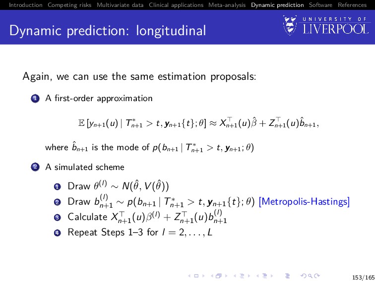
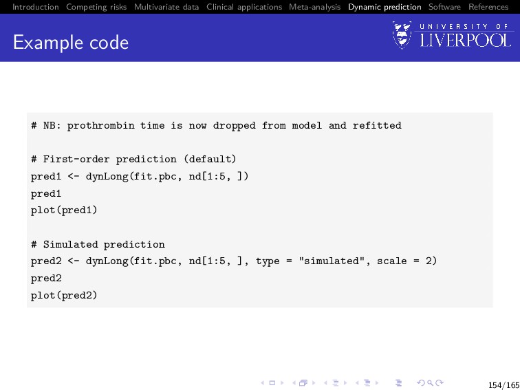
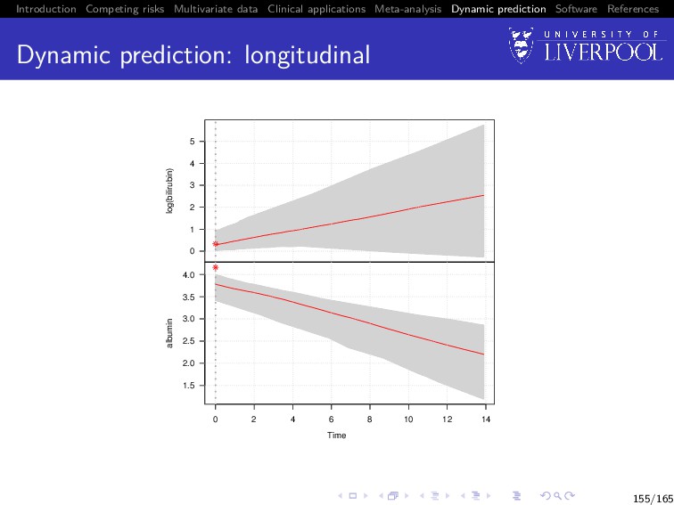
184. Introduction Competing risks Multivariate data Clinical applications Meta-analysis Dynamic prediction Software References Dynamic prediction: longitudinal For a new subject i = n + 1, we want to calculate E yn+1(u) | T∗ n+1 > t, yn+1{t}; θ = Xn+1 (u)β + Zn+1 (u)E[bn+1], 152/165
185. Introduction Competing risks Multivariate data Clinical applications Meta-analysis Dynamic prediction Software References Dynamic prediction: longitudinal Again, we can use the same estimation proposals: 1 A first-order approximation E [yn+1 (u) | T∗ n+1 > t, yn+1{t}; θ] ≈ Xn+1 (u)ˆ β + Zn+1 (u)ˆ bn+1, where ˆ bn+1 is the mode of p(bn+1 | T∗ n+1 > t, yn+1 ; θ) 2 A simulated scheme 1 Draw θ(l) ∼ N(ˆ θ, V (ˆ θ)) 2 Draw b(l) n+1 ∼ p(bn+1 | T∗ n+1 > t, yn+1{t}; θ) [Metropolis-Hastings] 3 Calculate Xn+1 (u)β(l) + Zn+1 (u)b(l) n+1 4 Repeat Steps 1–3 for l = 2, . . . , L 153/165
186. Introduction Competing risks Multivariate data Clinical applications Meta-analysis Dynamic prediction Software References Example code # NB: prothrombin time is now dropped from model and refitted # First-order prediction (default) pred1 <- dynLong(fit.pbc, nd[1:5, ]) pred1 plot(pred1) # Simulated prediction pred2 <- dynLong(fit.pbc, nd[1:5, ], type = "simulated", scale = 2) pred2 plot(pred2) 154/165
187. Introduction Competing risks Multivariate data Clinical applications Meta-analysis Dynamic prediction Software References Dynamic prediction: longitudinal 155/165 0 1 2 3 4 5 xpts log(bilirubin) 1.5 2.0 2.5 3.0 3.5 4.0 xpts albumin 0 2 4 6 8 10 12 14 Time
188. Introduction Competing risks Multivariate data Clinical applications Meta-analysis Dynamic prediction Software References Up next Lunch break — 1300–1345 Catch us at the break or lunch Software practical session — 1345–1630 156/165
189. Introduction Competing risks Multivariate data Clinical applications Meta-analysis Dynamic prediction Software References Software practical 157/165
190. Introduction Competing risks Multivariate data Clinical applications Meta-analysis Dynamic prediction Software References Software implementations in R Advanced statistical methods have limited use if not readily and publicly available in software R is a free software environment for statistical computing and graphics It compiles and runs on a wide variety of UNIX platforms, Windows, and macOS 158/165
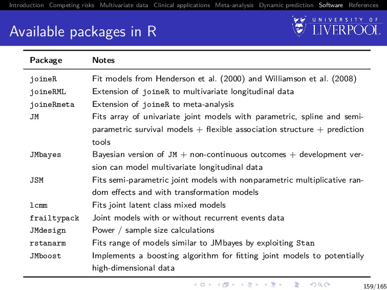
191. Introduction Competing risks Multivariate data Clinical applications Meta-analysis Dynamic prediction Software References Available packages in R Package Notes joineR Fit models from Henderson et al. (2000) and Williamson et al. (2008) joineRML Extension of joineR to multivariate longitudinal data joineRmeta Extension of joineR to meta-analysis JM Fits array of univariate joint models with parametric, spline and semi- parametric survival models + flexible association structure + prediction tools JMbayes Bayesian version of JM + non-continuous outcomes + development ver- sion can model multivariate longitudinal data JSM Fits semi-parametric joint models with nonparametric multiplicative ran- dom effects and with transformation models lcmm Fits joint latent class mixed models frailtypack Joint models with or without recurrent events data JMdesign Power / sample size calculations rstanarm Fits range of models similar to JMbayes by exploiting Stan JMboost Implements a boosting algorithm for fitting joint models to potentially high-dimensional data 159/165
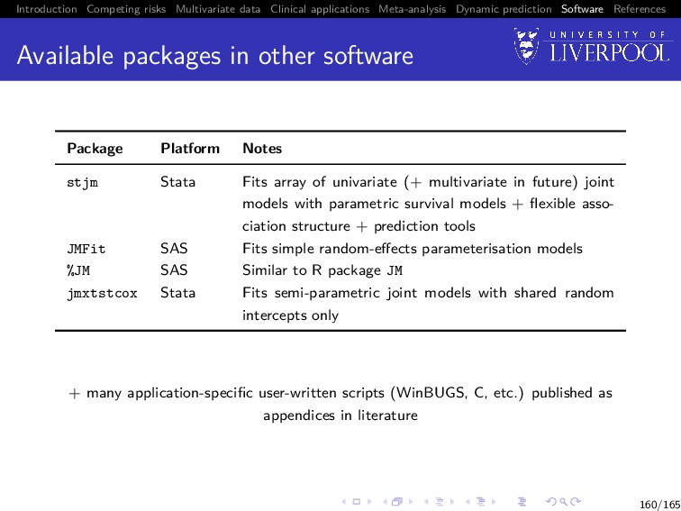
192. Introduction Competing risks Multivariate data Clinical applications Meta-analysis Dynamic prediction Software References Available packages in other software Package Platform Notes stjm Stata Fits array of univariate (+ multivariate in future) joint models with parametric survival models + flexible asso- ciation structure + prediction tools JMFit SAS Fits simple random-effects parameterisation models %JM SAS Similar to R package JM jmxtstcox Stata Fits semi-parametric joint models with shared random intercepts only + many application-specific user-written scripts (WinBUGS, C, etc.) published as appendices in literature 160/165
193. Introduction Competing risks Multivariate data Clinical applications Meta-analysis Dynamic prediction Software References Software we are using today +joineRmeta 161/165
194. Introduction Competing risks Multivariate data Clinical applications Meta-analysis Dynamic prediction Software References References I Henderson, Robin et al. (2000). Joint modelling of longitudinal measurements and event time data. Biostatistics 1(4), pp. 465–480. Pinheiro, Jos´ e C and Bates, Douglas M (2000). Mixed-Effects Models in S and S-PLUS. New York: Springer Verlag. Therneau, Terry M and Grambsch, Patricia M (2000). Modeling Survival Data: Extending the Cox Model. New Jersey: Springer-Verlag, p. 350. Andrinopoulou, Eleni-Rosalina et al. (2017). Combined dynamic predictions using joint models of two longitudinal outcomes and competing risk data. Statistical Methods in Medical Research 26(4), pp. 1787–1801. Xu, Jane and Zeger, Scott L (2001). The evaluation of multiple surrogate endpoints. Biometrics 57(1), pp. 81–87. Wulfsohn, M S and Tsiatis, Anastasios A (1997). A joint model for survival and longitudinal data measured with error. Biometrics 53(1), pp. 330–339. Laird, Nan M and Ware, James H (1982). Random-effects models for longitudinal data. Biometrics 38(4), pp. 963–74. 162/165
195. Introduction Competing risks Multivariate data Clinical applications Meta-analysis Dynamic prediction Software References References II Dempster, A P et al. (1977). Maximum likelihood from incomplete data via the EM algorithm. Journal of the Royal Statistical Society. Series B: Statistical Methodology 39(1), pp. 1–38. Hsieh, Fushing et al. (2006). Joint modeling of survival and longitudinal data: Likelihood approach revisited. Biometrics 62(4), pp. 1037–1043. Williamson, Paula R et al. (2008). Joint modelling of longitudinal and competing risks data. Statistics in Medicine 27, pp. 6426–6438. Murtaugh, Paul A et al. (1994). Primary biliary cirrhosis: prediction of short-term survival based on repeated patient visits. Hepatology 20(1), pp. 126–134. Hickey, Graeme L et al. (2016). Joint modelling of time-to-event and multivariate longitudinal outcomes: recent developments and issues. BMC Medical Research Methodology 16(1), pp. 1–15. Wei, Greg C. and Tanner, Martin A. (1990). A Monte Carlo implementation of the EM algorithm and the poor man’s data augmentation algorithms. Journal of the American Statistical Association 85(411), pp. 699–704. 163/165
196. Introduction Competing risks Multivariate data Clinical applications Meta-analysis Dynamic prediction Software References References III Ripatti, Samuli et al. (2002). Maximum likelihood inference for multivariate frailty models using an automated Monte Carlo EM algorithm. Lifetime Data Analysis 8(2002), pp. 349–360. McLachlan, Geoffrey J and Krishnan, Thriyambakam (2008). The EM Algorithm and Extensions. Second. Wiley-Interscience. Gueyffier, F. et al. (1995). INDANA: a meta-analysis on individual patient data in hypertension. Protocol and preliminary results. Therapie 50, pp. 353–362. Sudell, M. et al. (2017). Investigation of 2-stage meta–analysis methods for joint longitudinal and time-to-event data through simulation and real data application. Statistics in Medicine 37(8), pp. 1227–1244. DerSimonian, R. and Laird, N. (1986). Meta-analysis in clinical trials. Controlled Clinical Trials 7(3), pp. 177 –188. Rizopoulos, Dimitris (2011). Dynamic predictions and prospective accuracy in joint models for longitudinal and time-to-event data. Biometrics 67(3), pp. 819–829. 164/165
197. Introduction Competing risks Multivariate data Clinical applications Meta-analysis Dynamic prediction Software References References IV Therneau, Terry M and Watson, David A (2015). The concordance statistic and the Cox model. Tech. rep. Rochester, Minnesota: Department of Health Science Research, Mayo Clinic, Technical Report Series No. 85. 165/165