modelling of multivariate longitudinal and time-to-event data Graeme L. Hickey1, Pete Philipson2, Andrea Jorgensen1, Ruwanthi-Kolamunnage-Dona1 1Department of Biostatistics, University of Liverpool, UK 2Mathematics, Physics and Electrical Engineering, University of Northumbria, UK [email protected] Funded by Grant MR/M013227/1 13th November 2017 GL. Hickey Joint modelling of multivariate data 1 / 48
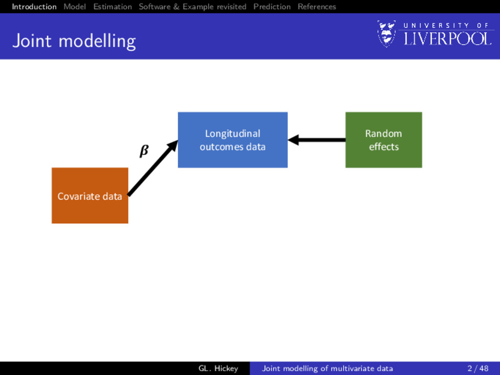
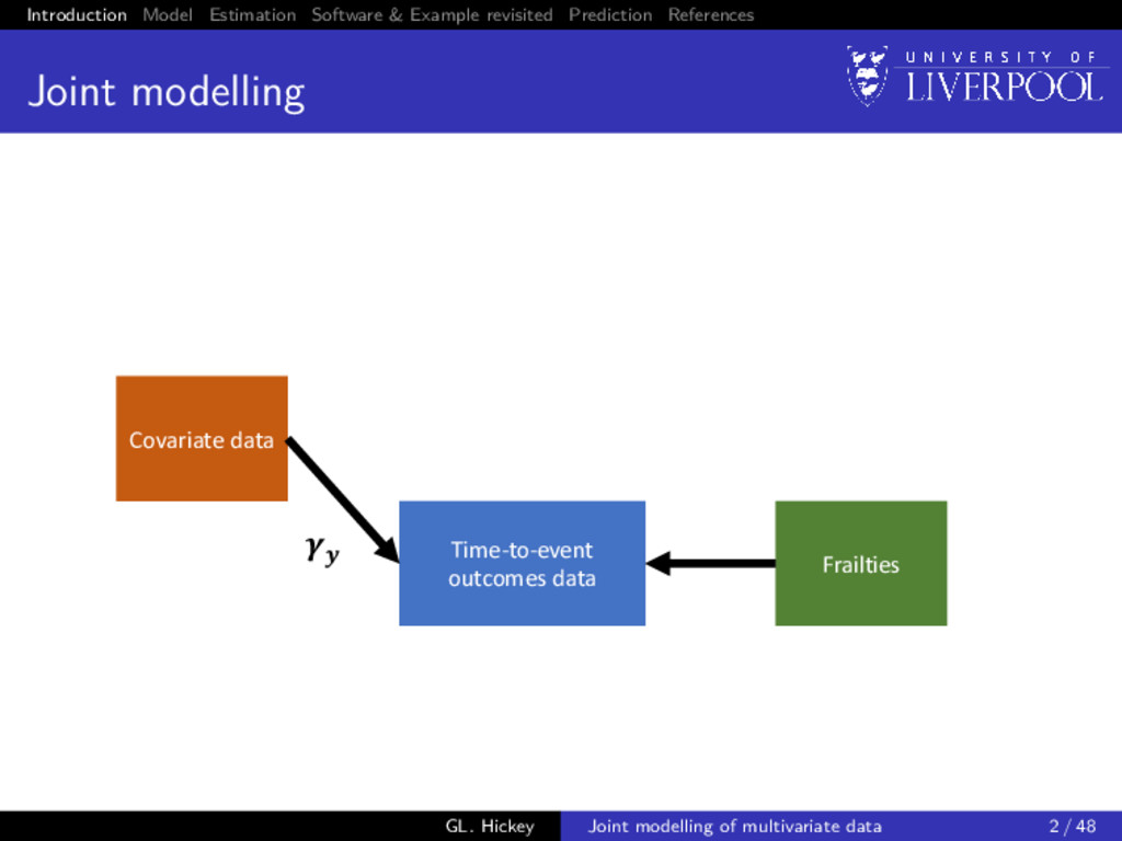
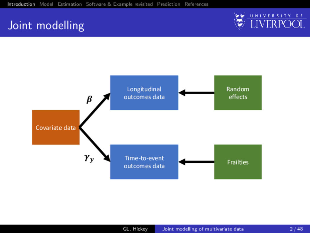
modelling Covariate data Time-to-event outcomes data Frailties Longitudinal outcomes data Random effects GL. Hickey Joint modelling of multivariate data 2 / 48
modelling Covariate data Time-to-event outcomes data Frailties Longitudinal outcomes data Random effects GL. Hickey Joint modelling of multivariate data 2 / 48
use a joint model? Interest lies with adjustment of inferences about longitudinal measurements for possibly outcome-dependent drop-out adjustment of inferences about the time-to-event distribution conditional on intermediate and/or error prone longitudinal measurements the joint evolution of the measurement and event time processes biomarker surrogacy dynamic prediction GL. Hickey Joint modelling of multivariate data 3 / 48
for multivariate joint models Clinical studies often repeatedly measure multiple biomarkers or other measurements and an event time Research has predominantly focused on a single event time and single measurement outcome Ignoring correlation leads to bias and reduced efficiency in estimation Harnessing all available information in a single model is advantageous and should lead to improved model predictions GL. Hickey Joint modelling of multivariate data 4 / 48
example Figure source: https://www.medgadget.com Primary biliary cirrhosis (PBC) is a chronic liver disease char- acterized by inflammatory de- struction of the small bile ducts, which eventually leads to cirrho- sis of the liver and death GL. Hickey Joint modelling of multivariate data 5 / 48
example Consider a subset of 154 patients randomized to placebo treatment from Mayo Clinic trial (Murtaugh et al. 1994) Multiple biomarkers repeatedly measured at intermittent times, of which we consider 3 clinically relevant ones: 1 serum bilirunbin (mg/dl) 2 serum albumin (mg/dl) 3 prothrombin time (seconds) GL. Hickey Joint modelling of multivariate data 6 / 48
1 1 Determine if longitudinal biomarker trajectories are associated with death Objective 2 1 Dynamically predict the biomarker trajectories and time to death for a new patient GL. Hickey Joint modelling of multivariate data 7 / 48
1 1 Determine if longitudinal biomarker trajectories are associated with death Objective 2 1 Dynamically predict the biomarker trajectories and time to death for a new patient Objective 3 1 Wrap it all up into a freely available software package GL. Hickey Joint modelling of multivariate data 7 / 48
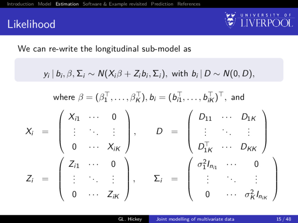
For each subject i = 1, . . . , n, we observe yi = (yi1 , . . . , yiK ) is a K-variate continuous outcome vector, where each yik denotes an (nik × 1)-vector of observed longitudinal measurements for the k-th outcome type: yik = (yi1k, . . . , yinik k) Observation times tijk for j = 1, . . . , nik, which can differ between subjects and outcomes (Ti , δi ), where Ti = min(T∗ i , Ci ), where T∗ i is the true event time, Ci corresponds to a potential right-censoring time, and δi is the failure indicator equal to 1 if the failure is observed (T∗ i ≤ Ci ) and 0 otherwise GL. Hickey Joint modelling of multivariate data 10 / 48
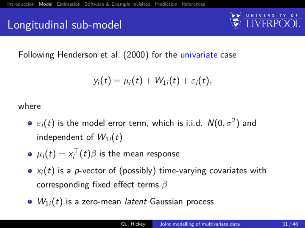
sub-model Following Henderson et al. (2000) for the univariate case yi (t) = µi (t) + W1i (t) + εi (t), where εi (t) is the model error term, which is i.i.d. N(0, σ2) and independent of W1i (t) µi (t) = xi (t)β is the mean response xi (t) is a p-vector of (possibly) time-varying covariates with corresponding fixed effect terms β W1i (t) is a zero-mean latent Gaussian process GL. Hickey Joint modelling of multivariate data 11 / 48
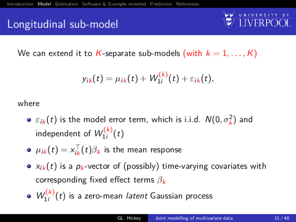
sub-model We can extend it to K-separate sub-models (with k = 1, . . . , K) yik(t) = µik(t) + W (k) 1i (t) + εik(t), where εik(t) is the model error term, which is i.i.d. N(0, σ2 k ) and independent of W (k) 1i (t) µik(t) = xik (t)βk is the mean response xik(t) is a pk-vector of (possibly) time-varying covariates with corresponding fixed effect terms βk W (k) 1i (t) is a zero-mean latent Gaussian process GL. Hickey Joint modelling of multivariate data 11 / 48
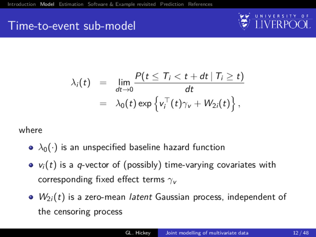
sub-model λi (t) = lim dt→0 P(t ≤ Ti < t + dt | Ti ≥ t) dt = λ0(t) exp vi (t)γv + W2i (t) , where λ0(·) is an unspecified baseline hazard function vi (t) is a q-vector of (possibly) time-varying covariates with corresponding fixed effect terms γv W2i (t) is a zero-mean latent Gaussian process, independent of the censoring process GL. Hickey Joint modelling of multivariate data 12 / 48
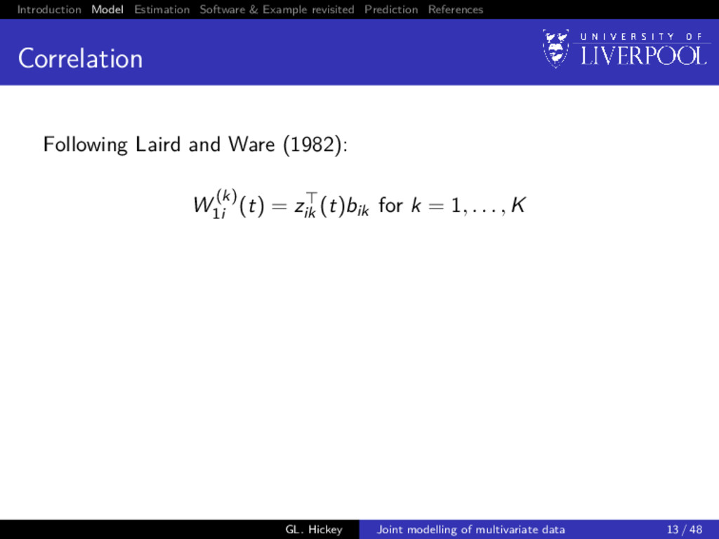
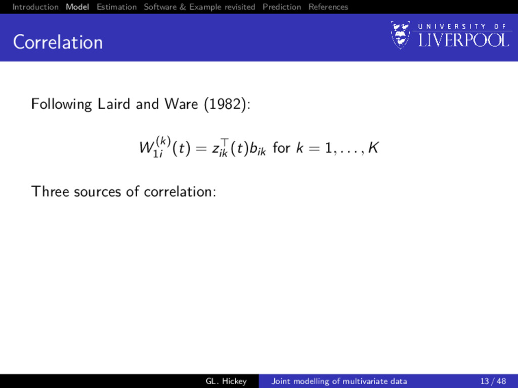
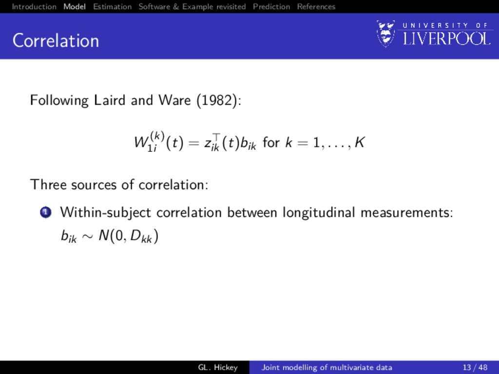
Following Laird and Ware (1982): W (k) 1i (t) = zik (t)bik for k = 1, . . . , K Three sources of correlation: GL. Hickey Joint modelling of multivariate data 13 / 48
Following Laird and Ware (1982): W (k) 1i (t) = zik (t)bik for k = 1, . . . , K Three sources of correlation: 1 Within-subject correlation between longitudinal measurements: bik ∼ N(0, Dkk) GL. Hickey Joint modelling of multivariate data 13 / 48
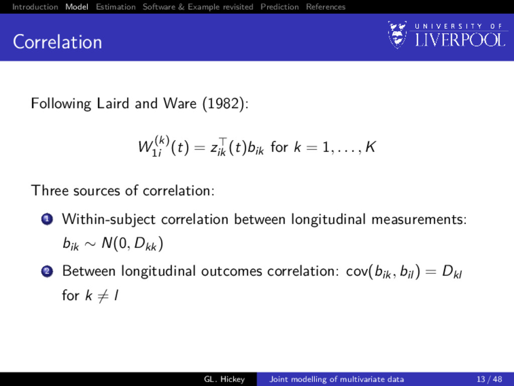
Following Laird and Ware (1982): W (k) 1i (t) = zik (t)bik for k = 1, . . . , K Three sources of correlation: 1 Within-subject correlation between longitudinal measurements: bik ∼ N(0, Dkk) 2 Between longitudinal outcomes correlation: cov(bik, bil ) = Dkl for k = l GL. Hickey Joint modelling of multivariate data 13 / 48
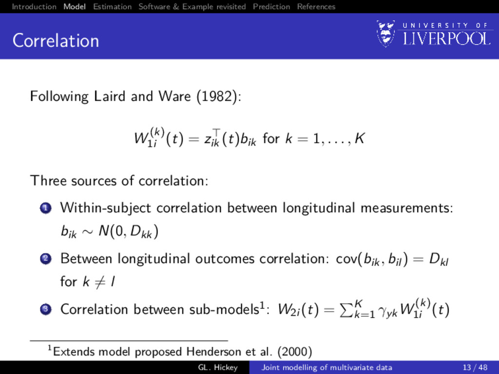
Following Laird and Ware (1982): W (k) 1i (t) = zik (t)bik for k = 1, . . . , K Three sources of correlation: 1 Within-subject correlation between longitudinal measurements: bik ∼ N(0, Dkk) 2 Between longitudinal outcomes correlation: cov(bik, bil ) = Dkl for k = l 3 Correlation between sub-models1: W2i (t) = K k=1 γykW (k) 1i (t) 1Extends model proposed Henderson et al. (2000) GL. Hickey Joint modelling of multivariate data 13 / 48
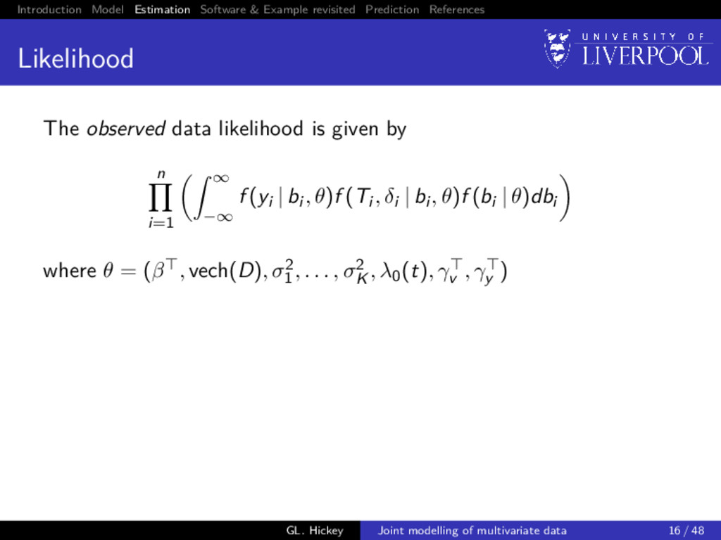
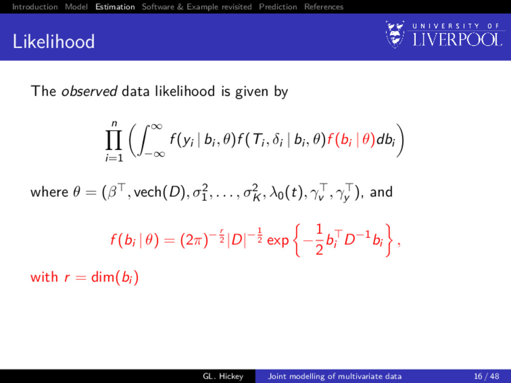
The observed data likelihood is given by n i=1 ∞ −∞ f (yi | bi , θ)f (Ti , δi | bi , θ)f (bi | θ)dbi where θ = (β , vech(D), σ2 1 , . . . , σ2 K , λ0(t), γv , γy ) GL. Hickey Joint modelling of multivariate data 16 / 48
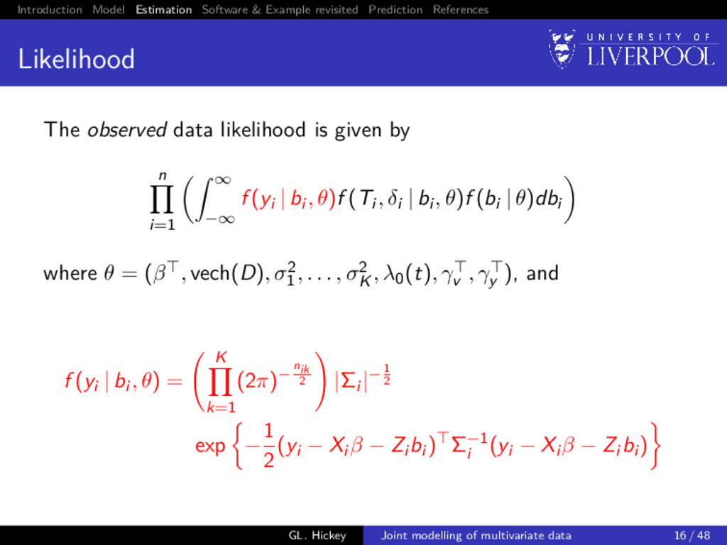
The observed data likelihood is given by n i=1 ∞ −∞ f (yi | bi , θ)f (Ti , δi | bi , θ)f (bi | θ)dbi where θ = (β , vech(D), σ2 1 , . . . , σ2 K , λ0(t), γv , γy ), and f (yi | bi , θ) = K k=1 (2π)−nik 2 |Σi |−1 2 exp − 1 2 (yi − Xi β − Zi bi ) Σ−1 i (yi − Xi β − Zi bi ) GL. Hickey Joint modelling of multivariate data 16 / 48
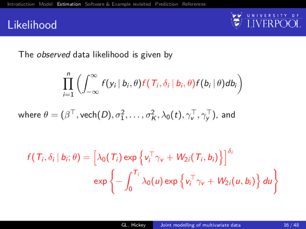
The observed data likelihood is given by n i=1 ∞ −∞ f (yi | bi , θ)f (Ti , δi | bi , θ)f (bi | θ)dbi where θ = (β , vech(D), σ2 1 , . . . , σ2 K , λ0(t), γv , γy ), and f (Ti , δi | bi ; θ) = λ0(Ti ) exp vi γv + W2i (Ti , bi ) δi exp − Ti 0 λ0(u) exp vi γv + W2i (u, bi ) du GL. Hickey Joint modelling of multivariate data 16 / 48
The observed data likelihood is given by n i=1 ∞ −∞ f (yi | bi , θ)f (Ti , δi | bi , θ)f (bi | θ)dbi where θ = (β , vech(D), σ2 1 , . . . , σ2 K , λ0(t), γv , γy ), and f (bi | θ) = (2π)− r 2 |D|−1 2 exp − 1 2 bi D−1bi , with r = dim(bi ) GL. Hickey Joint modelling of multivariate data 16 / 48
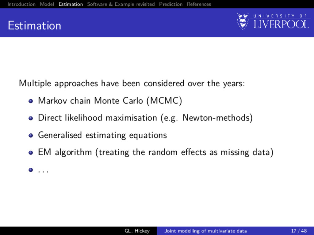
Multiple approaches have been considered over the years: Markov chain Monte Carlo (MCMC) Direct likelihood maximisation (e.g. Newton-methods) Generalised estimating equations EM algorithm (treating the random effects as missing data) . . . GL. Hickey Joint modelling of multivariate data 17 / 48
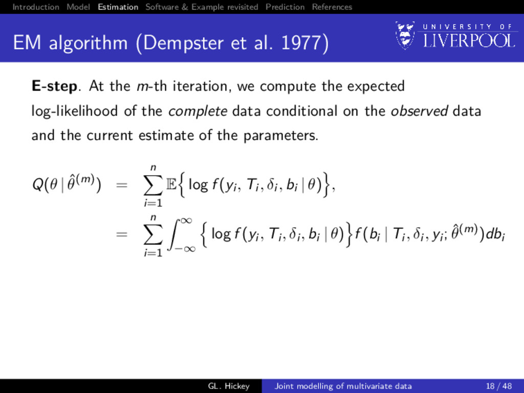
algorithm (Dempster et al. 1977) E-step. At the m-th iteration, we compute the expected log-likelihood of the complete data conditional on the observed data and the current estimate of the parameters. Q(θ | ˆ θ(m)) = n i=1 E log f (yi , Ti , δi , bi | θ) , = n i=1 ∞ −∞ log f (yi , Ti , δi , bi | θ) f (bi | Ti , δi , yi ; ˆ θ(m))dbi GL. Hickey Joint modelling of multivariate data 18 / 48
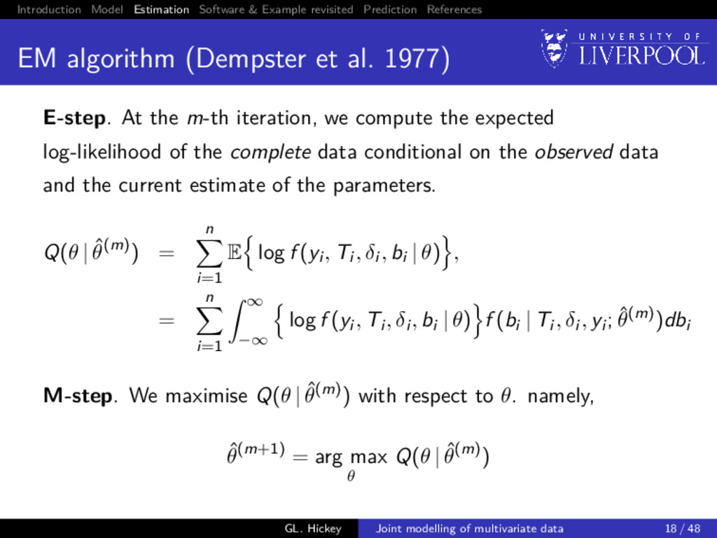
algorithm (Dempster et al. 1977) E-step. At the m-th iteration, we compute the expected log-likelihood of the complete data conditional on the observed data and the current estimate of the parameters. Q(θ | ˆ θ(m)) = n i=1 E log f (yi , Ti , δi , bi | θ) , = n i=1 ∞ −∞ log f (yi , Ti , δi , bi | θ) f (bi | Ti , δi , yi ; ˆ θ(m))dbi M-step. We maximise Q(θ | ˆ θ(m)) with respect to θ. namely, ˆ θ(m+1) = arg max θ Q(θ | ˆ θ(m)) GL. Hickey Joint modelling of multivariate data 18 / 48
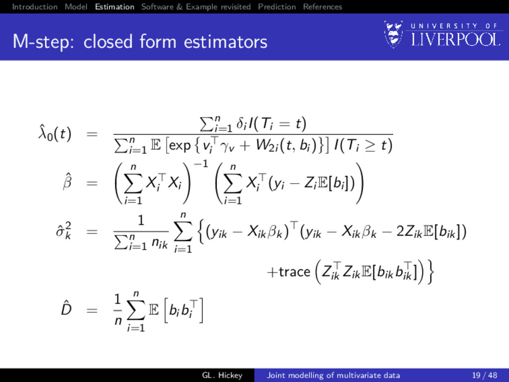
closed form estimators ˆ λ0(t) = n i=1 δi I(Ti = t) n i=1 E exp vi γv + W2i (t, bi ) I(Ti ≥ t) ˆ β = n i=1 Xi Xi −1 n i=1 Xi (yi − Zi E[bi ]) ˆ σ2 k = 1 n i=1 nik n i=1 (yik − Xikβk) (yik − Xikβk − 2ZikE[bik]) +trace Zik ZikE[bikbik ] ˆ D = 1 n n i=1 E bi bi GL. Hickey Joint modelling of multivariate data 19 / 48
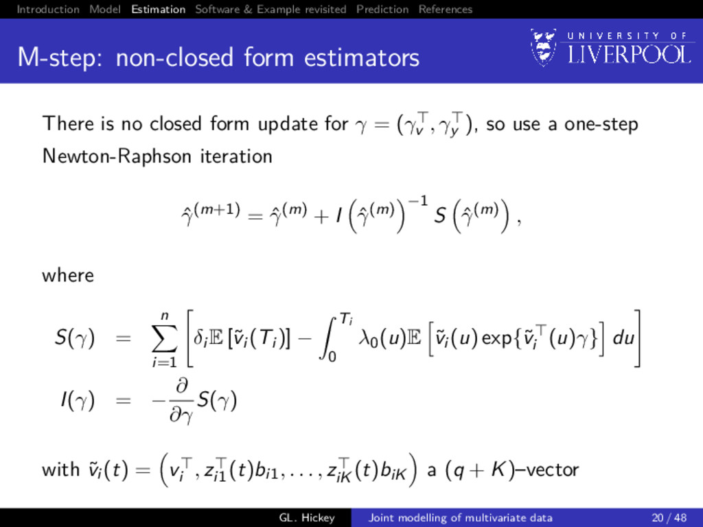
non-closed form estimators There is no closed form update for γ = (γv , γy ), so use a one-step Newton-Raphson iteration ˆ γ(m+1) = ˆ γ(m) + I ˆ γ(m) −1 S ˆ γ(m) , where S(γ) = n i=1 δi E [˜ vi (Ti )] − Ti 0 λ0(u)E ˜ vi (u) exp{˜ vi (u)γ} du I(γ) = − ∂ ∂γ S(γ) with ˜ vi (t) = vi , zi1 (t)bi1, . . . , ziK (t)biK a (q + K)–vector GL. Hickey Joint modelling of multivariate data 20 / 48
algorithm E-step requires calculating several multidimensional integrals of form E h(bi ) | Ti , δi , yi ; ˆ θ Gauss-quadrature can be slow if dim(bi ) is large ⇒ might not scale well as K increases Instead, we use the Monte Carlo Expectation-Maximization (MCEM; Wei and Tanner 1990) M-step updates remain the same GL. Hickey Joint modelling of multivariate data 21 / 48
Carlo E-step Conventional EM algorithm: use quadrature to compute E h(bi ) | Ti , δi , yi ; ˆ θ = ∞ −∞ h(bi )f (bi | yi ; ˆ θ)f (Ti , δi | bi ; ˆ θ)dbi ∞ −∞ f (bi | yi ; ˆ θ)f (Ti , δi | bi ; ˆ θ)dbi , where h(·) = any known fuction, bi | yi , θ ∼ N Ai Zi Σ−1 i (yi − Xi β) , Ai , and Ai = Zi Σ−1 i Zi + D−1 −1 GL. Hickey Joint modelling of multivariate data 22 / 48
Carlo E-step MCEM algorithm E-step: use Monte Carlo integration to compute E h(bi ) | Ti , δi , yi ; ˆ θ ≈ 1 N N d=1 h b(d) i f Ti , δi | b(d) i ; ˆ θ 1 N N d=1 f Ti , δi | b(d) i ; ˆ θ where h(·) = any known fuction, bi | yi , θ ∼ N Ai Zi Σ−1 i (yi − Xi β) , Ai , and Ai = Zi Σ−1 i Zi + D−1 −1 b(1) i , b(2) i , . . . , b(N) i ∼ bi | yi , θ a Monte Carlo draw GL. Hickey Joint modelling of multivariate data 22 / 48
up convergence Monte Carlo integration converges at a rate of O(N−1/2), which is independent of K and r = dim(bi ) EM algorithm convergences linearly Can we speed this up? GL. Hickey Joint modelling of multivariate data 23 / 48
up convergence Monte Carlo integration converges at a rate of O(N−1/2), which is independent of K and r = dim(bi ) EM algorithm convergences linearly Can we speed this up? 1 Antithetic variates 2 Quasi-Monte Carlo GL. Hickey Joint modelling of multivariate data 23 / 48
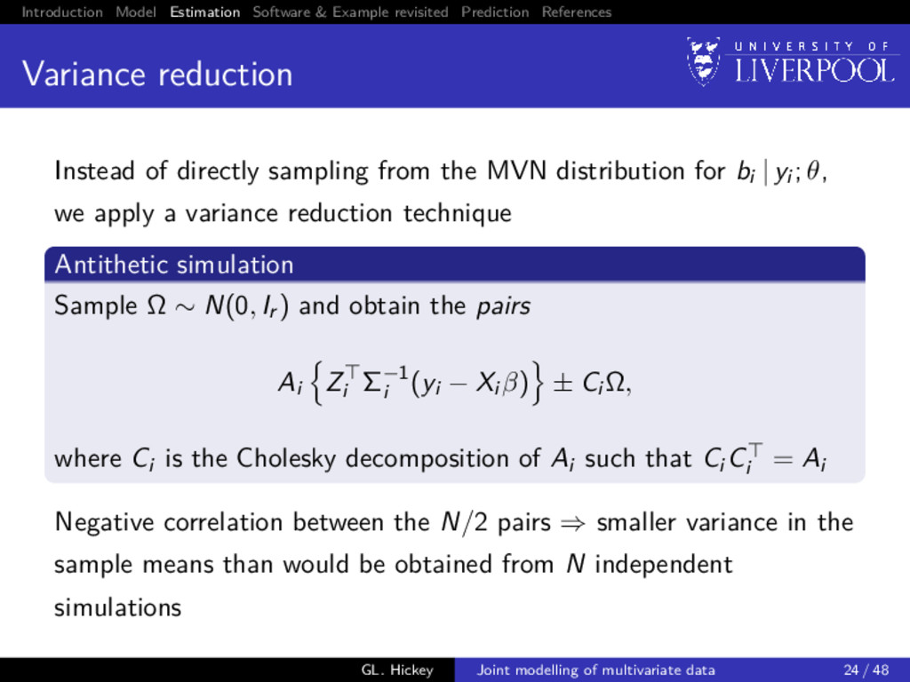
reduction Instead of directly sampling from the MVN distribution for bi | yi ; θ, we apply a variance reduction technique Antithetic simulation Sample Ω ∼ N(0, Ir ) and obtain the pairs Ai Zi Σ−1 i (yi − Xi β) ± Ci Ω, where Ci is the Cholesky decomposition of Ai such that Ci Ci = Ai Negative correlation between the N/2 pairs ⇒ smaller variance in the sample means than would be obtained from N independent simulations GL. Hickey Joint modelling of multivariate data 24 / 48
In standard EM, convergence usually declared at (m + 1)-th iteration if one of the following criteria satisfied Relative change: ∆(m+1) rel = max |ˆ θ(m+1)−ˆ θ(m)| |ˆ θ(m)|+ 1 < 0 Absolute change: ∆(m+1) abs = max |ˆ θ(m+1) − ˆ θ(m)| < 2 for some choice of 0, 1, and 2 GL. Hickey Joint modelling of multivariate data 25 / 48
In MCEM framework, there are 2 complications to account for 1 spurious convergence declared due to random chance GL. Hickey Joint modelling of multivariate data 26 / 48
In MCEM framework, there are 2 complications to account for 1 spurious convergence declared due to random chance ⇒ Solution: require convergence for 3 iterations in succession GL. Hickey Joint modelling of multivariate data 26 / 48
In MCEM framework, there are 2 complications to account for 1 spurious convergence declared due to random chance ⇒ Solution: require convergence for 3 iterations in succession 2 estimators swamped by Monte Carlo error, thus precluding convergence GL. Hickey Joint modelling of multivariate data 26 / 48
In MCEM framework, there are 2 complications to account for 1 spurious convergence declared due to random chance ⇒ Solution: require convergence for 3 iterations in succession 2 estimators swamped by Monte Carlo error, thus precluding convergence ⇒ Solution: increase Monte Carlo size N as algorithm moves closer towards maximizer GL. Hickey Joint modelling of multivariate data 26 / 48
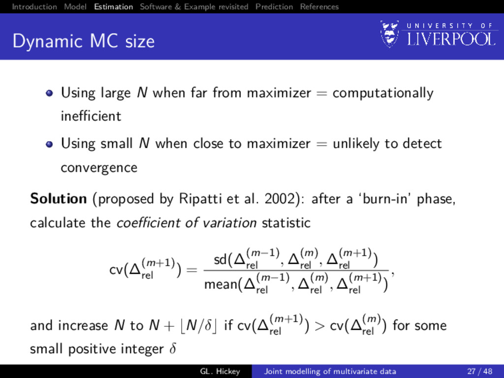
MC size Using large N when far from maximizer = computationally inefficient Using small N when close to maximizer = unlikely to detect convergence Solution (proposed by Ripatti et al. 2002): after a ‘burn-in’ phase, calculate the coefficient of variation statistic cv(∆(m+1) rel ) = sd(∆(m−1) rel , ∆(m) rel , ∆(m+1) rel ) mean(∆(m−1) rel , ∆(m) rel , ∆(m+1) rel ) , and increase N to N + N/δ if cv(∆(m+1) rel ) > cv(∆(m) rel ) for some small positive integer δ GL. Hickey Joint modelling of multivariate data 27 / 48
Carlo Replaces the (pseudo-)random sequence by a deterministic one Quasi-random sequences yield smaller errors than standard Monte Carlo integration methods Convergence is O (logN)r N Research on-going. . . GL. Hickey Joint modelling of multivariate data 28 / 48
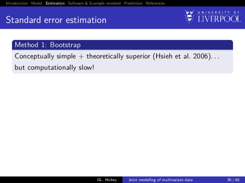
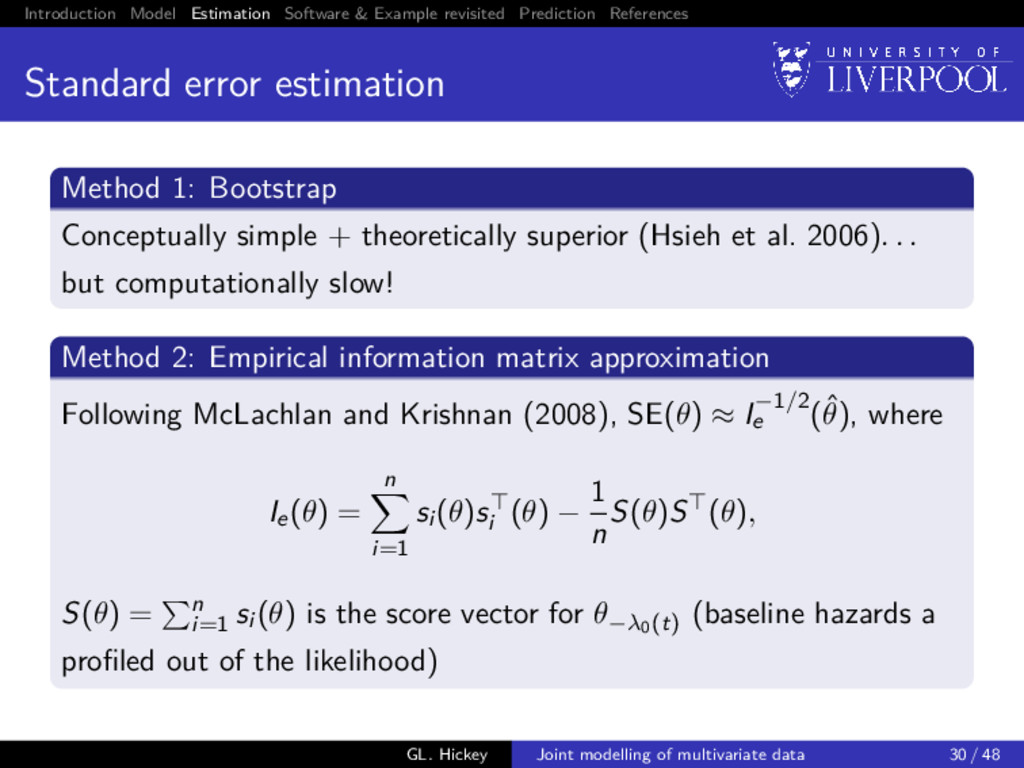
error estimation Method 1: Bootstrap Conceptually simple + theoretically superior (Hsieh et al. 2006). . . but computationally slow! Method 2: Empirical information matrix approximation Following McLachlan and Krishnan (2008), SE(θ) ≈ I−1/2 e (ˆ θ), where Ie(θ) = n i=1 si (θ)si (θ) − 1 n S(θ)S (θ), S(θ) = n i=1 si (θ) is the score vector for θ−λ0(t) (baseline hazards a profiled out of the likelihood) GL. Hickey Joint modelling of multivariate data 30 / 48
options Pre-2017: none! 2017-onwards: joineRML: discussed today stjm: a new extension to the Stata package2 written by Michael Crowther megenreg: similar to stjm, but can handle other models rstanarm: development branch that absorbs package written by Sam Brilleman3 JMbayes: a new extension4 to the R package written by Dimitris Rizopoulos 2Crowther MJ. Joint Statistical Meeting. Seattle; 2015. 3 github.com/sambrilleman/rstanjm 4 github.com/drizopoulos/JMbayes GL. Hickey Joint modelling of multivariate data 32 / 48
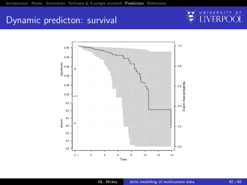
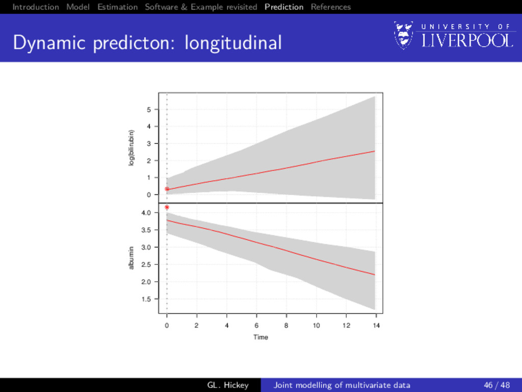
prediction So far we have only discussed inference from joint models How we can use them for prediction? Predict what? 1 Failure probability at time u > t given longitudinal data observed up until time t 2 Longitudinal trajectories at time u > t given longitudinal data observed up until time t GL. Hickey Joint modelling of multivariate data 37 / 48
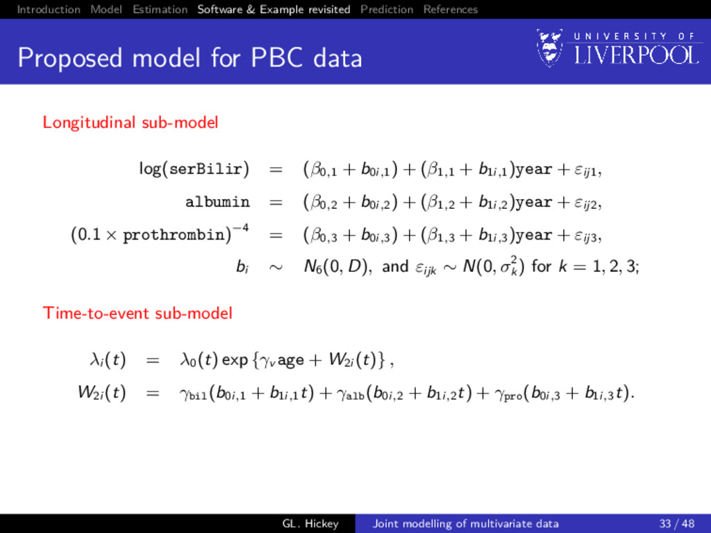
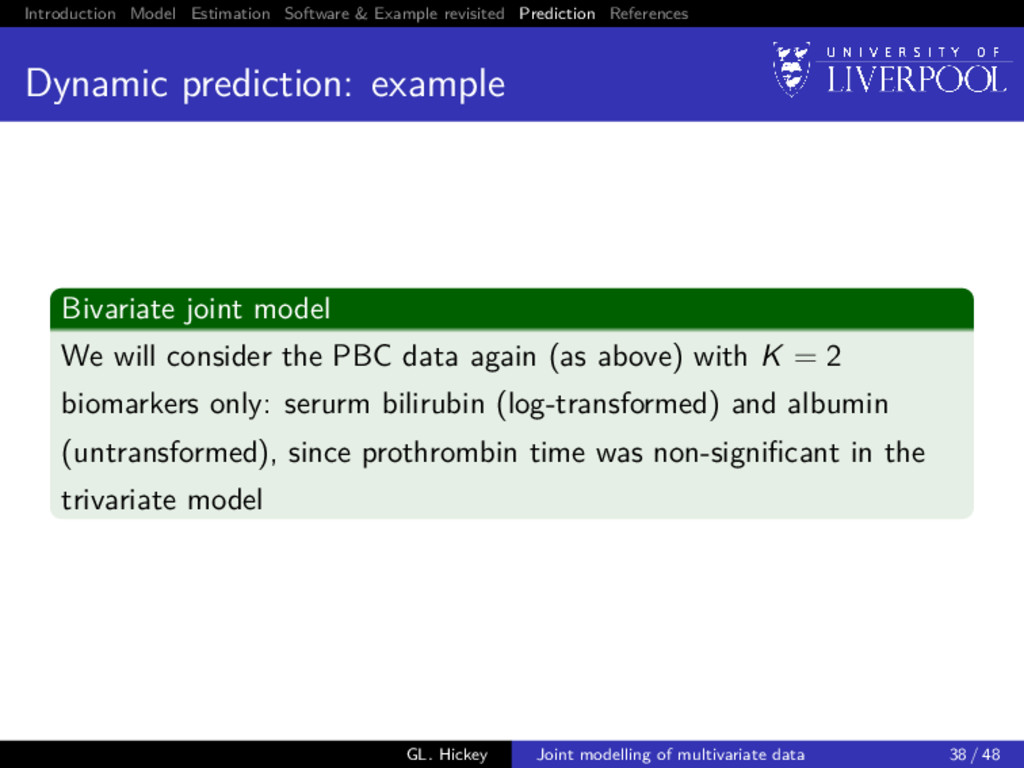
prediction: example Bivariate joint model We will consider the PBC data again (as above) with K = 2 biomarkers only: serurm bilirubin (log-transformed) and albumin (untransformed), since prothrombin time was non-significant in the trivariate model GL. Hickey Joint modelling of multivariate data 38 / 48
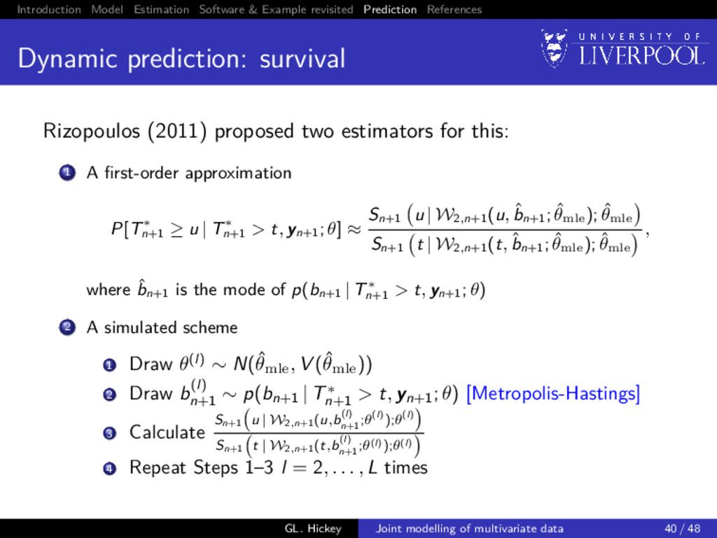
prediction: survival For a new subject i = n + 1, we want to calculate P[T∗ n+1 ≥ u | T∗ n+1 > t, yn+1; θ] = E Sn+1 (u | W2,n+1(u, bn+1; θ); θ) Sn+1 (t | W2,n+1(t, bn+1; θ); θ) , where W2i (t, bi ; θ) = {W2i (s, vi ; θ); 0 ≤ s < t} and the expectation is taken with respect to the distribution p(bn+1 | T∗ n+1 > t, yn+1; θ) GL. Hickey Joint modelling of multivariate data 39 / 48
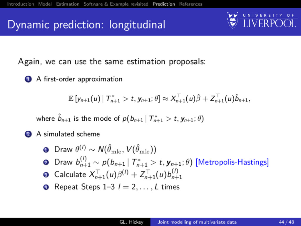
prediction: longitudinal For a new subject i = n + 1, we want to calculate E yn+1(u) | T∗ n+1 > t, yn+1; θ = Xn+1 (u)β + Zn+1 (u)E[bn+1], GL. Hickey Joint modelling of multivariate data 43 / 48
challenges How can we incorporate high-dimensional K? E.g. K = 10? Data reduction techniques: can we project high-dimensional K onto a lower order plane? Speed-up calculations using approximations (e.g. Laplace approximations) GL. Hickey Joint modelling of multivariate data 47 / 48
Murtaugh, Paul A et al. (1994). Primary biliary cirrhosis: prediction of short-term survival based on repeated patient visits. Hepatology 20(1), pp. 126–134. Henderson, R et al. (2000). Joint modelling of longitudinal measurements and event time data. Biostatistics 1(4), pp. 465–480. Laird, NM and Ware, JH (1982). Random-effects models for longitudinal data. Biometrics 38(4), pp. 963–74. Dempster, AP et al. (1977). Maximum likelihood from incomplete data via the EM algorithm. J Roy Stat Soc B 39(1), pp. 1–38. Wei, GC and Tanner, MA (1990). A Monte Carlo implementation of the EM algorithm and the poor man’s data augmentation algorithms. J Am Stat Assoc 85(411), pp. 699–704. Ripatti, S et al. (2002). Maximum likelihood inference for multivariate frailty models using an automated Monte Carlo EM algorithm. Life Dat Anal 8(2002), pp. 349–360. Hsieh, F et al. (2006). Joint modeling of survival and longitudinal data: Likelihood approach revisited. Biometrics 62(4), pp. 1037–1043. McLachlan, GJ and Krishnan, T (2008). The EM Algorithm and Extensions. Second. Wiley-Interscience. Rizopoulos, Dimitris (2011). Dynamic predictions and prospective accuracy in joint models for longitudinal and time-to-event data. Biometrics 67(3), pp. 819–829. GL. Hickey Joint modelling of multivariate data 48 / 48