Dynamic survival prediction for multivariate joint models using the R package joineRML
Presented at the 10th International Conference of the ERCIM WG on Computational and Methodological Statistics (CMStatistics 2017), Senate House , University of London, UK, 16-18 December
survival prediction for multivariate joint models using the R package joineRML Graeme L. Hickey1, Pete Philipson2, Andrea Jorgensen1, Ruwanthi Kolamunnage-Dona1 1Department of Biostatistics, University of Liverpool, UK 2Mathematics, Physics and Electrical Engineering, University of Northumbria, UK [email protected] 17th December 2017 GL. Hickey Joint modelling of multivariate data 1 / 28
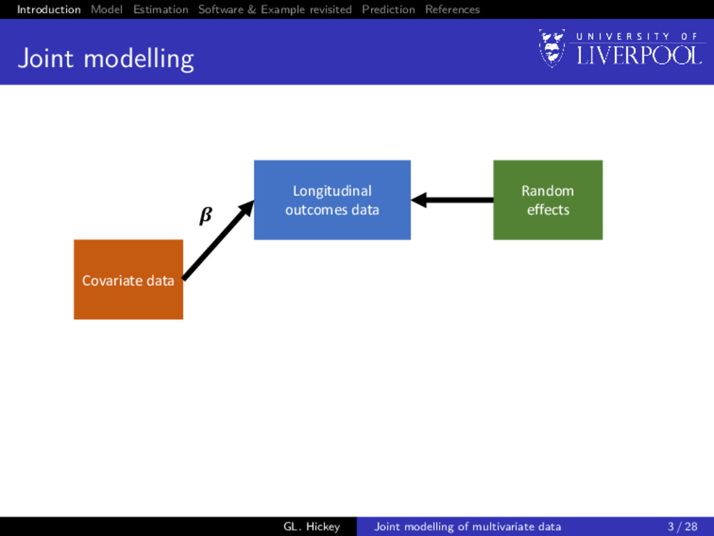
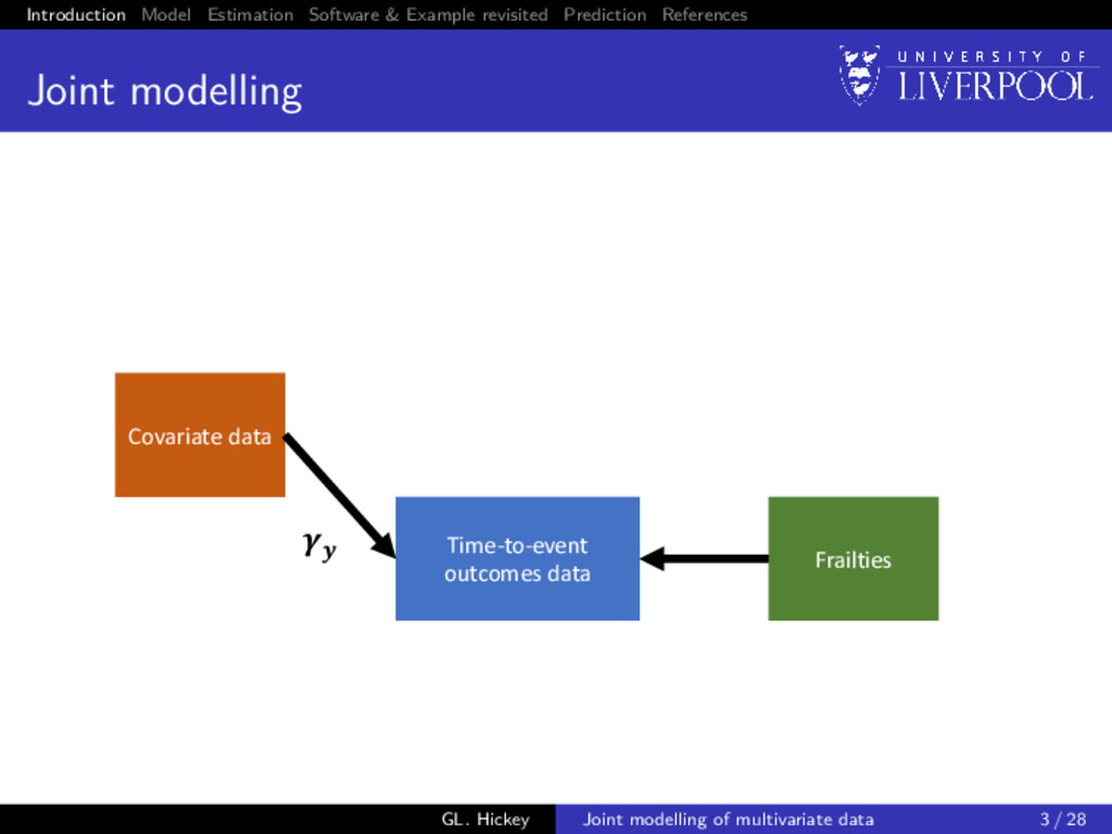
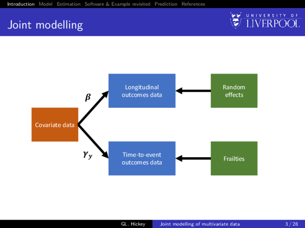
modelling Covariate data Time-to-event outcomes data Frailties Longitudinal outcomes data Random effects GL. Hickey Joint modelling of multivariate data 3 / 28
modelling Covariate data Time-to-event outcomes data Frailties Longitudinal outcomes data Random effects GL. Hickey Joint modelling of multivariate data 3 / 28
modelling Typically used for inference, but growing interest in using for dynamic prediction Typically used with a single longitudinal outcome, but growing interest in using multiple (or multivariate) longitudinal outcomes We will describe a recent –package that resolves these two issues GL. Hickey Joint modelling of multivariate data 4 / 28
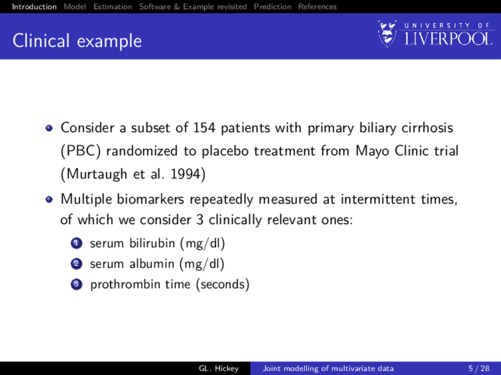
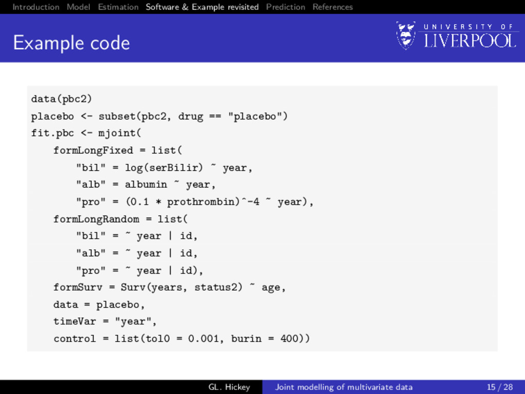
example Consider a subset of 154 patients with primary biliary cirrhosis (PBC) randomized to placebo treatment from Mayo Clinic trial (Murtaugh et al. 1994) Multiple biomarkers repeatedly measured at intermittent times, of which we consider 3 clinically relevant ones: 1 serum bilirubin (mg/dl) 2 serum albumin (mg/dl) 3 prothrombin time (seconds) GL. Hickey Joint modelling of multivariate data 5 / 28
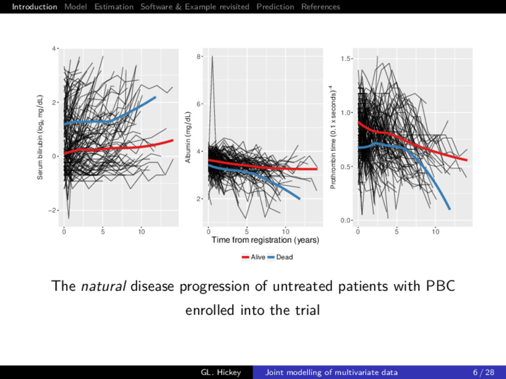
time (0.1 x seconds)−4 Albumin (mg dL) Serum bilirubin (loge mg dL) 0 5 10 0 5 10 0 5 10 0.0 0.5 1.0 1.5 2 4 6 8 −2 0 2 4 Time from registration (years) Alive Dead The natural disease progression of untreated patients with PBC enrolled into the trial GL. Hickey Joint modelling of multivariate data 6 / 28
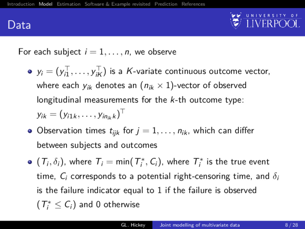
For each subject i = 1, . . . , n, we observe yi = (yi1 , . . . , yiK ) is a K-variate continuous outcome vector, where each yik denotes an (nik × 1)-vector of observed longitudinal measurements for the k-th outcome type: yik = (yi1k, . . . , yinik k) Observation times tijk for j = 1, . . . , nik, which can differ between subjects and outcomes (Ti , δi ), where Ti = min(T∗ i , Ci ), where T∗ i is the true event time, Ci corresponds to a potential right-censoring time, and δi is the failure indicator equal to 1 if the failure is observed (T∗ i ≤ Ci ) and 0 otherwise GL. Hickey Joint modelling of multivariate data 8 / 28
sub-model We extend the univariate joint model from Henderson et al. (2000): yik(t) = xik (t)βk + zik (t)bik + εik(t), with k = 1, . . . , K where xik(t) is a pk-vector of (possibly) time-varying covariates with corresponding fixed effect terms βk bik ∼ N(0, Dkk) subject-and-marker specific random effects cov(bik, bil ) = Dkl for k = l εik(t) is the model error term, which is i.i.d. N(0, σ2 k ) and independent of bik GL. Hickey Joint modelling of multivariate data 9 / 28
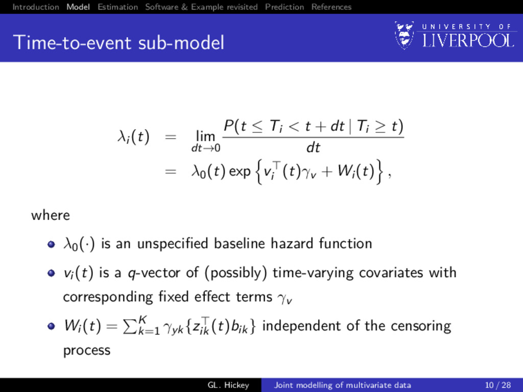
sub-model λi (t) = lim dt→0 P(t ≤ Ti < t + dt | Ti ≥ t) dt = λ0(t) exp vi (t)γv + Wi (t) , where λ0(·) is an unspecified baseline hazard function vi (t) is a q-vector of (possibly) time-varying covariates with corresponding fixed effect terms γv Wi (t) = K k=1 γyk{zik (t)bik} independent of the censoring process GL. Hickey Joint modelling of multivariate data 10 / 28
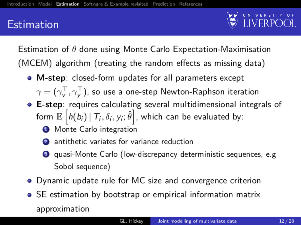
Estimation of θ done using Monte Carlo Expectation-Maximisation (MCEM) algorithm (treating the random effects as missing data) M-step: closed-form updates for all parameters except γ = (γv , γy ), so use a one-step Newton-Raphson iteration E-step: requires calculating several multidimensional integrals of form E h(bi ) | Ti , δi , yi ; ˆ θ , which can be evaluated by: 1 Monte Carlo integration 2 antithetic variates for variance reduction 3 quasi-Monte Carlo (low-discrepancy deterministic sequences, e.g Sobol sequence) Dynamic update rule for MC size and convergence criterion SE estimation by bootstrap or empirical information matrix approximation GL. Hickey Joint modelling of multivariate data 12 / 28
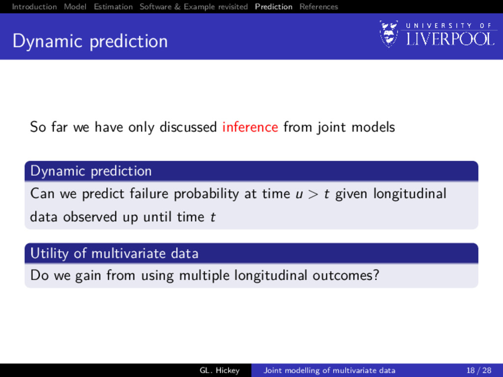
prediction So far we have only discussed inference from joint models Dynamic prediction Can we predict failure probability at time u > t given longitudinal data observed up until time t Utility of multivariate data Do we gain from using multiple longitudinal outcomes? GL. Hickey Joint modelling of multivariate data 18 / 28
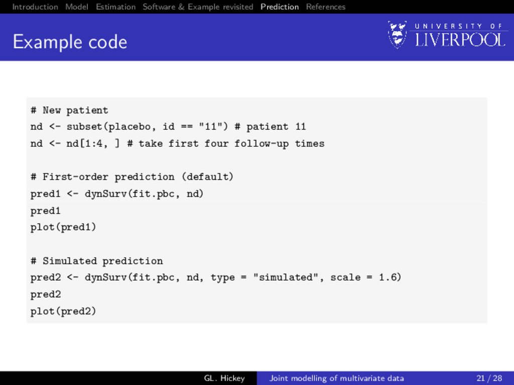
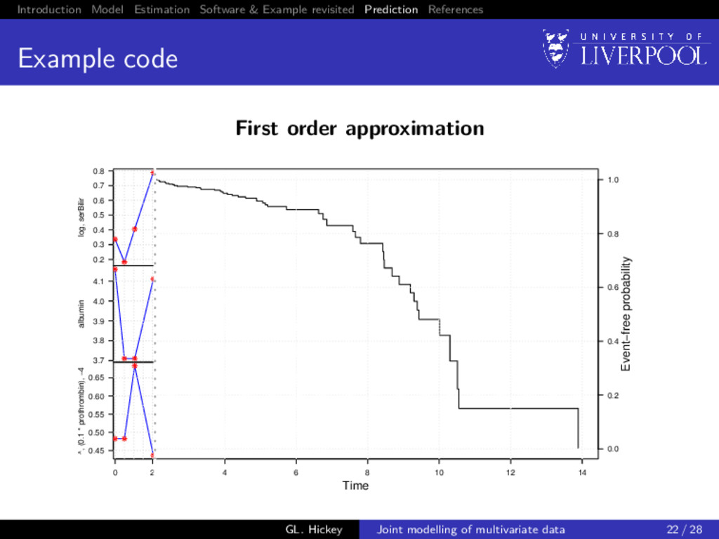
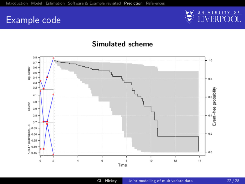
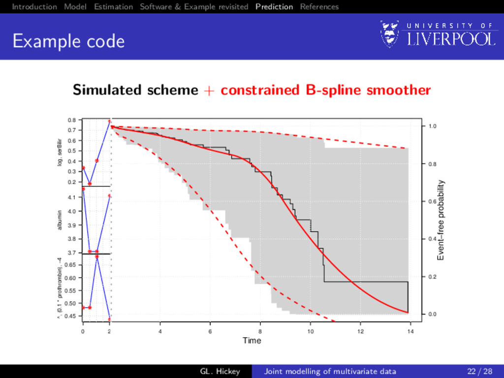
prediction For a new subject i = n + 1 with available longitudinal measurements yn+1{t} up to time t, we want to calculate P[T∗ n+1 ≥ u | T∗ n+1 > t, yn+1{t}; θ] = E Sn+1 (u | bn+1; θ) Sn+1 (t | bn+1; θ) , where the expectation is taken with respect to the distribution p(bn+1 | T∗ n+1 > t, yn+1{t}; θ), and Sn+1 (u | bn+1; θ) = exp − u 0 λ0(s) exp{vn+1 (s)γv + Wn+1(s)}ds GL. Hickey Joint modelling of multivariate data 19 / 28
software for dynamic prediction R (JM): univariate joint models (spline model for λ0(t)) 0 2 4 6 8 10 12 14 0.0 0.2 0.4 0.6 0.8 1.0 Univariate joint model {B} Time Pr(Ti ≥ u | Ti > t, y ~ i (t)) R package JM joineRML 0 2 4 6 8 10 12 14 0.0 0.2 0.4 0.6 0.8 1.0 Univariate joint model {A} Time Pr(Ti ≥ u | Ti > t, y ~ i (t)) R package JM joineRML 0 2 4 6 8 10 12 14 0.0 0.2 0.4 0.6 0.8 1.0 Univariate joint model {P} Time Pr(Ti ≥ u | Ti > t, y ~ i (t)) R package JM joineRML R (JMbayes): uni- and multi-variate joint models Stata (stjm): univariate joint models GL. Hickey Joint modelling of multivariate data 24 / 28
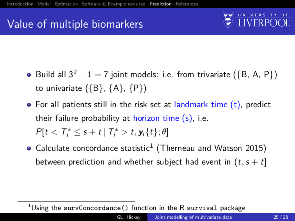
of multiple biomarkers Build all 32 − 1 = 7 joint models: i.e. from trivariate ({B, A, P}) to univariate ({B}, {A}, {P}) For all patients still in the risk set at landmark time (t), predict their failure probability at horizon time (s), i.e. P[t < T∗ i ≤ s + t | T∗ i > t, yi {t}; θ] Calculate concordance statistic1 (Therneau and Watson 2015) between prediction and whether subject had event in (t, s + t] 1Using the survConcordance() function in the R survival package GL. Hickey Joint modelling of multivariate data 25 / 28
Questions? Murtaugh, Paul A et al. (1994). Primary biliary cirrhosis: prediction of short-term survival based on repeated patient visits. Hepatology 20(1), pp. 126–134. Henderson, R et al. (2000). Joint modelling of longitudinal measurements and event time data. Biostatistics 1(4), pp. 465–480. Rizopoulos, Dimitris (2011). Dynamic predictions and prospective accuracy in joint models for longitudinal and time-to-event data. Biometrics 67(3), pp. 819–829. Therneau, Terry M and Watson, David A (2015). The concordance statistic and the Cox model. Tech. rep. Rochester, Minnesota: Department of Health Science Research, Mayo Clinic, Technical Report Series No. 85. GL. Hickey Joint modelling of multivariate data 28 / 28