What you need to know about statistics to read a journal article

EACTS Fundamentals in Cardiac Surgery: Part III

Transcript

1. What you need to know about statistics to read a journal article Graeme L. Hickey @graemeleehickey www.glhickey.com graeme.hickey@liverpool.ac.uk
2. Who am I? • Statistician (Ph.D. 2011, CStat 2016) • Former UK National Adult Cardiac Surgery Audit Statistician (2012-14) • Researcher who has published in cardiothoracic journals • Assistant Editor (Statistical Consultant) for the EJCTS and ICVTS (2012— present) 900 papers reviewed to-date
3. Statistics for surgeons • We use statistical methods we will use to transform complex raw data into meaningful results • We live in a world of evidence-based medicine, and statistics is the lingua franca • Choice of statistical methods will depend on several things, including: – Clinical question – Study design – Outcomes
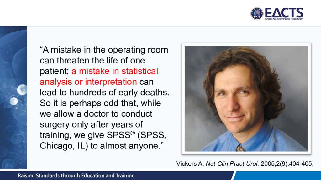
4. “A mistake in the operating room can threaten the life of one patient; a mistake in statistical analysis or interpretation can lead to hundreds of early deaths. So it is perhaps odd that, while we allow a doctor to conduct surgery only after years of training, we give SPSS® (SPSS, Chicago, IL) to almost anyone.” Vickers A. Nat Clin Pract Urol. 2005;2(9):404-405.
5. What is the study type? Clinical Practice Guidelines Meta-Analysis Systematic Review Randomized Controlled Trial Prospective, tests treatment Cohort Studies Prospective - exposed cohort is observed for outcome Case Control Studies Retrospective: subjects already of interest looking for risk factors Case Report or Case Series Narrative Reviews, Expert Opinions, Editorials Animal and Laboratory Studies No humans involved No design Observational Studies Primary Studies Secondary, pre- appraised, or filtered ANOVA Basic summary statistics Multivariable regression Propensity score methods RCT design Meta-analysis Figure source: https://en.wikipedia.org/wiki/Wikipedia:Identifying_reliable_sources_(medicine)
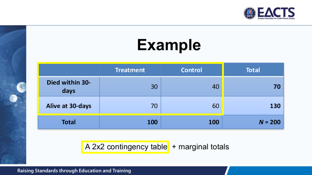
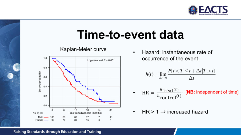
6. What are the study outcomes? • Continuous – E.g. volume of blood transfused after surgery • Dichotomous / binary – E.g. 30-day mortality status (dead versus alive) • Time-to-event – E.g. time from surgery to death or re-intervention • Ordinal – E.g. MV regurgitation grade at 12-months post-surgery • Count – E.g. number of infections in first post-treatment year
7. Interpretation of clinical trials
8. Descriptive statistics • Summarizing a binary outcome: “In-hospital mortality was 3.4% (3 / 87)” • Summarizing a continuous outcome: “The average length of postoperative stay [PLOS] was…” • 5 patients [PLOS: 3, 3, 4, 5, 90-days] • Mean: 21-days • Median: 4-days • Skew-distributions are more informatively summarised using quantiles: – Median (middle quartile) – (Lower (first) quartile, Upper (third) quartile) captures the variability
9. Relative vs. absolute effects Source: http://www.independent.co.uk/news/science/vitamin- d-asthma-attacks-prevent-study-cochrane-a7226756.html Source: https://www.theguardian.com/society/2016/sep/05/vitamin- d-supplements-could-halve-risk-of-serious-asthma-attacks Absolute risk Relative risk
10. Example Randomization N = 200 Treatment n = 100 Control n = 100 Dead at 30-days n = 30 Alive at 30-days n = 70 Dead at 30-days n = 40 Alive at 30-days n = 60
11. Example Treatment Control Total Died within 30- days 30 40 70 Alive at 30-days 70 60 130 Total 100 100 N = 200 A 2x2 contingency table + marginal totals
12. Example Treatment Control Total Died within 30- days a b a + b Alive at 30-days c d c + d Total a + c b + d N = a + b + c + d A 2x2 contingency table + marginal totals
13. Example Absolute risk in treatment group (ARtreat ) = + = 30 100 = 0.30 Absolute risk in control group (ARcontrol ) = + = 40 100 = 0.40 Absolute risk reduction (ARR) = ARcontrol − ARtreat = 0.4 − 0.3 = 0.10 Relative risk (RR) = ARtreat ARcontrol = 0.3 0.4 = 0.75 Relative risk reduction (RRR) = 1 − RR = 1 − 0.75 = 0.25 Source: http://clinicalevidence.bmj.com/x/set/static/ebm/learn/665075.html
14. 0.4 0.2 0.04 0.3 0.15 0.03 0 0.05 0.1 0.15 0.2 0.25 0.3 0.35 0.4 0.45 High risk Intermediate risk Low risk Results from 3 hypothetical RCTs of the same treatment Control Treatment 30-day mortality proportion High risk ARR = 0.1 RRR = 0.25 Intermediate risk ARR = 0.05 RRR = 0.25 Low risk ARR = 0.01 RRR = 0.25 Clinical importance depends on underlying prevalence
15. Example: ROOBY trial It is always preferable to report both the absolute and relative effect sizes Source: Lamy et al. N Engl J Med 2016; 375:2359-2368
16. Odds ratio vs. relative risk • Often confused with RR • Exaggerate treatment effect • Example: OR = 34 56 = 0.64 (recall: RR = 0.75) • OR ≈ RR for low baseline risk • Why do we use them? – Logistic regression – RRs precluded in some study designs (e.g. case-control) – ORdeath = 1 / ORsurvival (not for RRs) Source: Grant RL. BMJ, 2014; 348(4), f7450.
17. Time-to-event data • Hazard: instantaneous rate of occurrence of the event • HR = 9treat(?) 9control(?) • HR > 1 ⇒ increased hazard 800 1000 5 0.0 0.2 0.4 0.6 0.8 1.0 0 6 12 18 24 30 Time from diagnosis (months) Survival probability Male Female 138 86 35 17 7 2 90 70 30 15 6 1 No. at risk + + + + + + + ++ + + + + + ++ + + + + + + + + ++ + + + + + + + ++ + + ++ + ++ + + + + + + ++ + + + + + + Log−rank test P = 0.001 Kaplan-Meier curve [NB: independent of time]
18. Time-to-event data Relative effect: HR = 0.55 Absolute effect: ARR(12-months) = 20.0% 30.7% in the TAVI group 50.7% in the standard therapy group • HR uses all data at each time point • Not robust to departures from proportionality Source: Makkar et al. N Engl J Med 2012; 366:1696-1704.
19. Errors No evidence of a difference Evidence of a difference No difference True negative False positive Type I error () Difference False negative Type II error (β) True positive Truth Hypothesis test
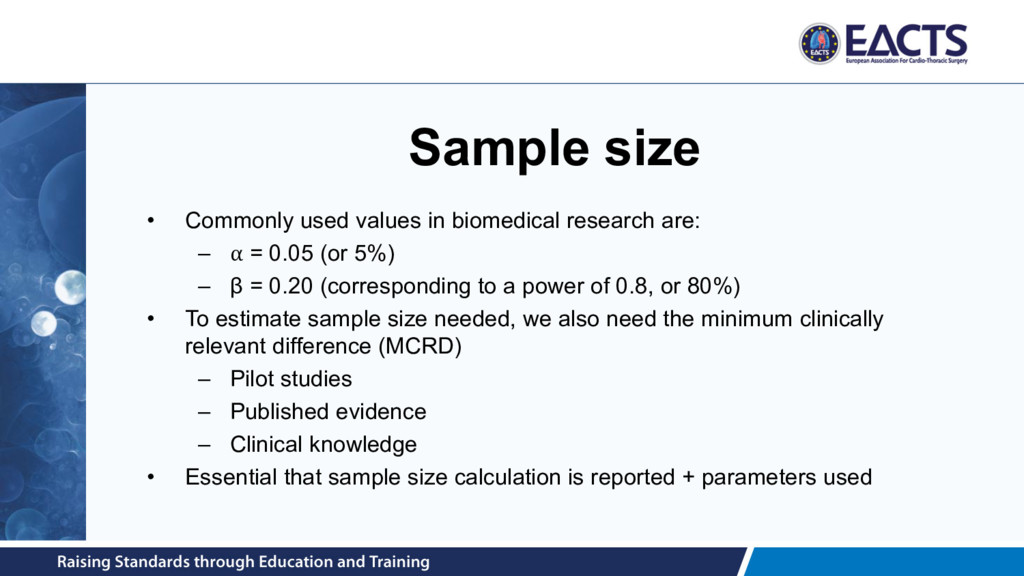
20. Sample size • Commonly used values in biomedical research are: – ⍺ = 0.05 (or 5%) – β = 0.20 (corresponding to a power of 0.8, or 80%) • To estimate sample size needed, we also need the minimum clinically relevant difference (MCRD) – Pilot studies – Published evidence – Clinical knowledge • Essential that sample size calculation is reported + parameters used
21. Choosing a statistical test • Need to know: – Continuous, discrete (dichotomous / categorical), or time-to-event data? – Independent or paired data? – Data satisfy test assumptions?
22. If distributional assumptions satisfied If distributional assumptions not satisfied
23. Source: Guller & DeLong. J Am Coll Surg. 2004;198(3):441-58.
24. Source: Guller & DeLong. J Am Coll Surg. 2004;198(3):441-58.
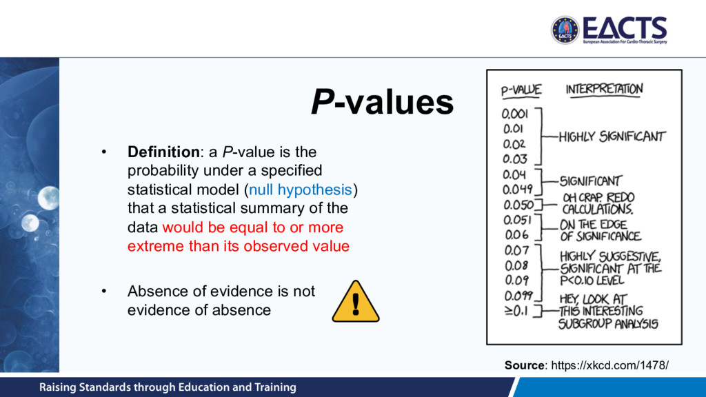
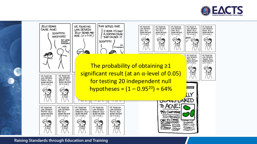
25. P-values • Definition: a P-value is the probability under a specified statistical model (null hypothesis) that a statistical summary of the data would be equal to or more extreme than its observed value • Absence of evidence is not evidence of absence Source: https://xkcd.com/1478/
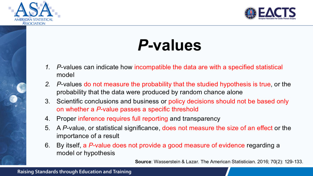
26. P-values 1. P-values can indicate how incompatible the data are with a specified statistical model 2. P-values do not measure the probability that the studied hypothesis is true, or the probability that the data were produced by random chance alone 3. Scientific conclusions and business or policy decisions should not be based only on whether a P-value passes a specific threshold 4. Proper inference requires full reporting and transparency 5. A P-value, or statistical significance, does not measure the size of an effect or the importance of a result 6. By itself, a P-value does not provide a good measure of evidence regarding a model or hypothesis Source: Wasserstein & Lazar. The American Statistician. 2016; 70(2): 129-133.
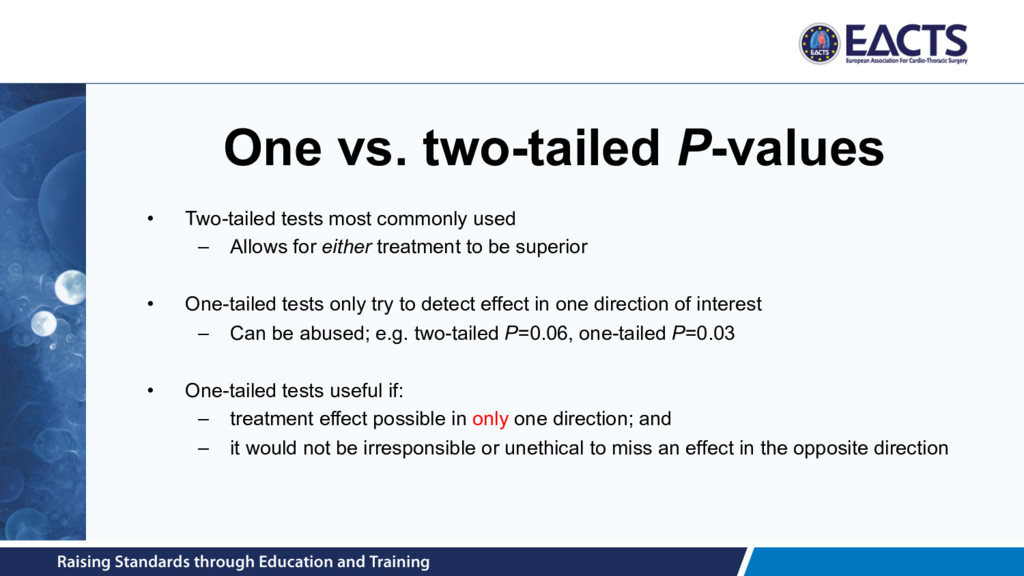
27. One vs. two-tailed P-values • Two-tailed tests most commonly used – Allows for either treatment to be superior • One-tailed tests only try to detect effect in one direction of interest – Can be abused; e.g. two-tailed P=0.06, one-tailed P=0.03 • One-tailed tests useful if: – treatment effect possible in only one direction; and – it would not be irresponsible or unethical to miss an effect in the opposite direction
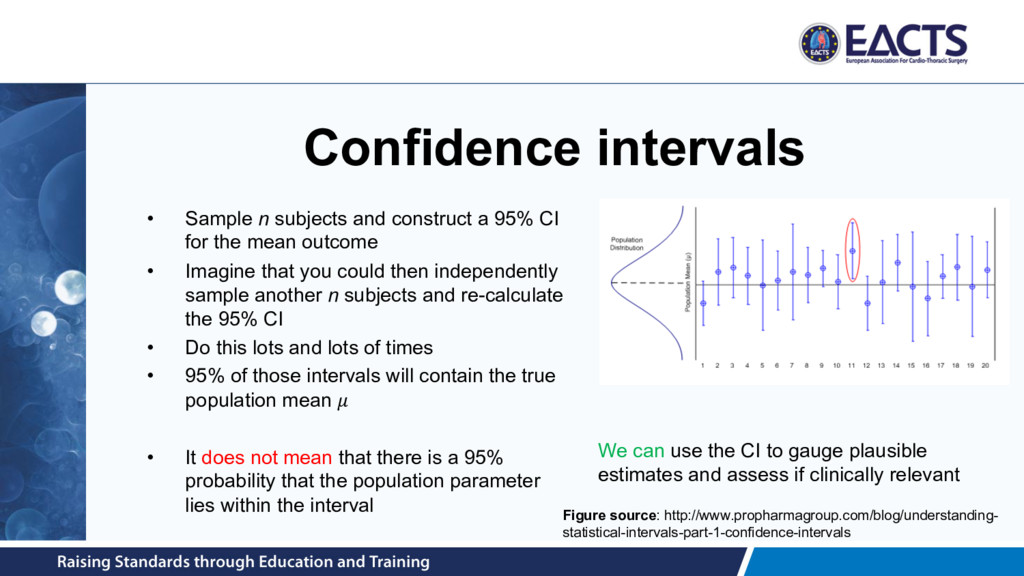
28. Confidence intervals • Sample n subjects and construct a 95% CI for the mean outcome • Imagine that you could then independently sample another n subjects and re-calculate the 95% CI • Do this lots and lots of times • 95% of those intervals will contain the true population mean • It does not mean that there is a 95% probability that the population parameter lies within the interval We can use the CI to gauge plausible estimates and assess if clinically relevant Figure source: http://www.propharmagroup.com/blog/understanding- statistical-intervals-part-1-confidence-intervals
29. Clinical vs. statistical significance • P-values become smaller as sample size increase • Which is more clinically significant? – Length of stay recorded for n patients randomized to open or EVAR surgery – Scenario 1: n = 16, difference 1-day (SD = 1-days) P=0.065 – Scenario 2: n = 2000, difference = 0.1-days (SD = 1-day); P=0.026 • Clinical significance ≠ statistical significance • Interpret the confidence interval rather than the P-value
30. Multiple comparisons & subgroup analyses • Similar issues • Each involves testing multiple hypotheses
31. The probability of obtaining ≥1 significant result (at an ⍺-level of 0.05) for testing 20 independent null hypotheses = (1 – 0.9520) = 64%
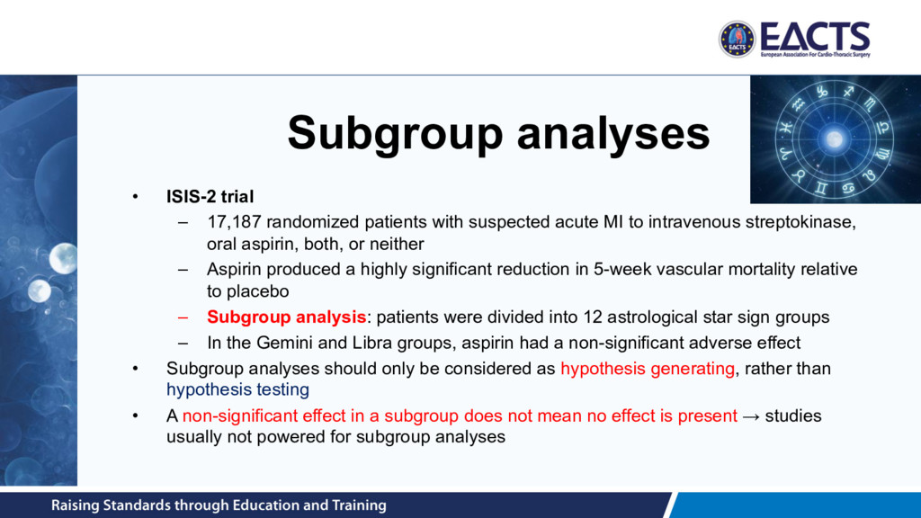
32. Subgroup analyses • ISIS-2 trial – 17,187 randomized patients with suspected acute MI to intravenous streptokinase, oral aspirin, both, or neither – Aspirin produced a highly significant reduction in 5-week vascular mortality relative to placebo – Subgroup analysis: patients were divided into 12 astrological star sign groups – In the Gemini and Libra groups, aspirin had a non-significant adverse effect • Subgroup analyses should only be considered as hypothesis generating, rather than hypothesis testing • A non-significant effect in a subgroup does not mean no effect is present → studies usually not powered for subgroup analyses
33. Many other statistical issues • Trial design – Superiority – Non-inferiority • Randomization methods • Outcome definitions – Composite or individual components • Cross-overs • Losses after randomization • Interim analyses • + many non-statistical issues
34. Observational studies
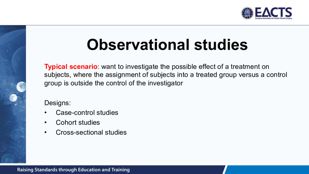
35. Observational studies Typical scenario: want to investigate the possible effect of a treatment on subjects, where the assignment of subjects into a treated group versus a control group is outside the control of the investigator Designs: • Case-control studies • Cohort studies • Cross-sectional studies
36. Example: MVR Source: Dimarakis et al. Heart 2014;100:500–507
37. Example: MVR In-hospital mortality: • Biological prosthesis group: 7.8% (152/1945) • Mechanical prosthesis group: 5.5% (106/1917) • P = 0.005 (chi square test) What is your conclusion (and why)?
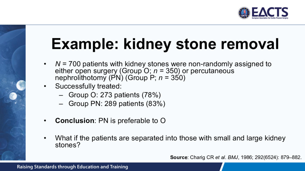
38. Example: kidney stone removal • N = 700 patients with kidney stones were non-randomly assigned to either open surgery (Group O; n = 350) or percutaneous nephrolithotomy (PN) (Group P; n = 350) • Successfully treated: – Group O: 273 patients (78%) – Group PN: 289 patients (83%) • Conclusion: PN is preferable to O • What if the patients are separated into those with small and large kidney stones? Source: Charig CR et al. BMJ, 1986; 292(6524): 879–882.
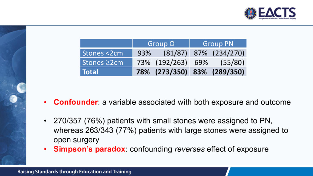
39. Group O Group PN Stones <2cm 93% (81/87) 87% (234/270) Stones ³2cm 73% (192/263) 69% (55/80) Total 78% (273/350) 83% (289/350) • Confounder: a variable associated with both exposure and outcome • 270/357 (76%) patients with small stones were assigned to PN, whereas 263/343 (77%) patients with large stones were assigned to open surgery • Simpson’s paradox: confounding reverses effect of exposure
40. d (or Δ) = the standardized difference (or bias) |Δ| > 0.1 (10%) represents meaningful imbalance in a given covariate between treatment groups
41. Example: MVR • Dimarakis et al. undertook 2 separate analyses: – Multivariable regression – Propensity score matching
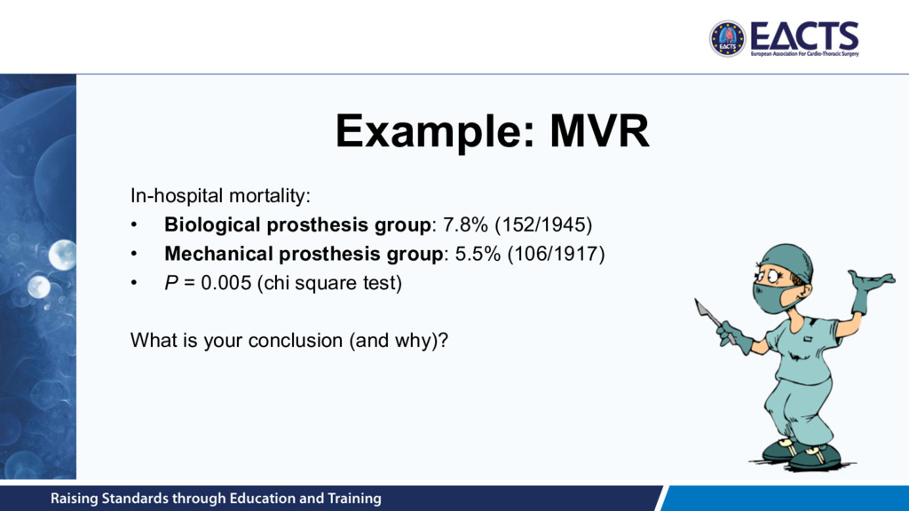
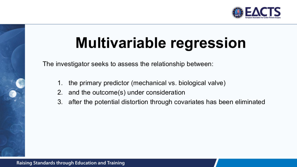
42. Multivariable regression The investigator seeks to assess the relationship between: 1. the primary predictor (mechanical vs. biological valve) 2. and the outcome(s) under consideration 3. after the potential distortion through covariates has been eliminated
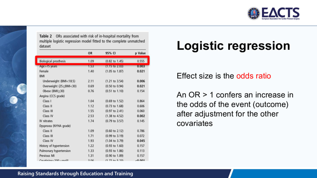
43. Regression models Outcome Model* β coefficient (for unit increase) Continuous (e.g. aneurysm diameter) Multiple linear regression Expected increase in outcome Binary (e.g. in-hospital mortality) Multiple logistic regression Log odds ratio Time-to-event (e.g. time to all-cause mortality) Multiple Cox proportional hazards regression Log hazard ratio *Other regression models exist as well
44. Logistic regression Effect size is the odds ratio An OR > 1 confers an increase in the odds of the event (outcome) after adjustment for the other covariates
45. Cox regression Effect size is the hazard ratio A HR > 1 confers an increase in the hazard of the event (outcome) after adjustment for the other covariates
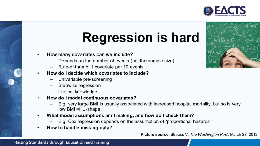
46. Regression is hard • How many covariates can we include? – Depends on the number of events (not the sample size) – Rule-of-thumb: 1 covariate per 10 events • How do I decide which covariates to include? – Univariable pre-screening – Stepwise regression – Clinical knowledge • How do I model continuous covariates? – E.g. very large BMI is usually associated with increased hospital mortality, but so is very low BMI ⇒ U-shape • What model assumptions am I making, and how do I check them? – E.g. Cox regression depends on the assumption of “proportional hazards” • How to handle missing data? Picture source: Strauss V. The Washington Post. March 27, 2013
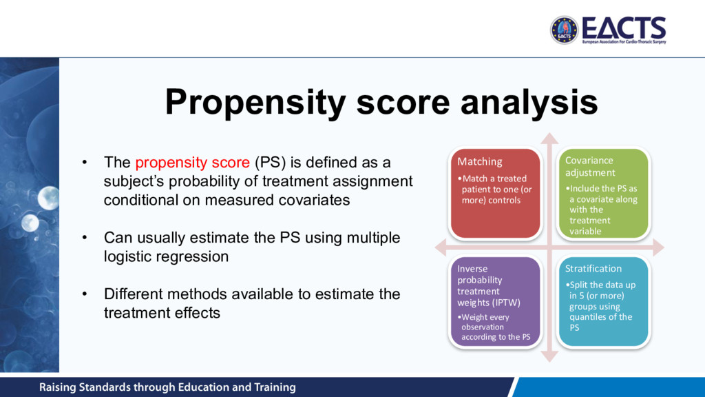
47. Propensity score analysis Matching •Match a treated patient to one (or more) controls Covariance adjustment •Include the PS as a covariate along with the treatment variable Inverse probability treatment weights (IPTW) •Weight every observation according to the PS Stratification •Split the data up in 5 (or more) groups using quantiles of the PS • The propensity score (PS) is defined as a subject’s probability of treatment assignment conditional on measured covariates • Can usually estimate the PS using multiple logistic regression • Different methods available to estimate the treatment effects
48. Propensity score matching Source: Dimarakis et al. Heart 2014;100:500–507.
49. Propensity score matching Source: Dimarakis et al. Heart 2014;100:500–507.
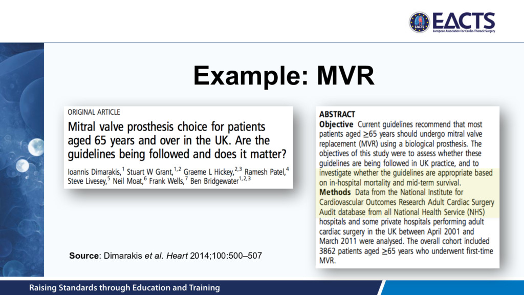
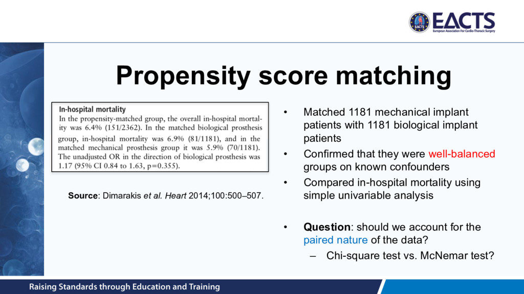
50. Propensity score matching • Matched 1181 mechanical implant patients with 1181 biological implant patients • Confirmed that they were well-balanced groups on known confounders • Compared in-hospital mortality using simple univariable analysis • Question: should we account for the paired nature of the data? – Chi-square test vs. McNemar test? Source: Dimarakis et al. Heart 2014;100:500–507.
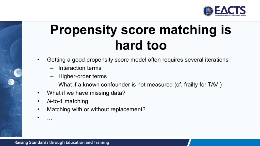
51. Propensity score matching is hard too • Getting a good propensity score model often requires several iterations – Interaction terms – Higher-order terms – What if a known confounder is not measured (cf. frailty for TAVI) • What if we have missing data? • N-to-1 matching • Matching with or without replacement? • …
52. Evidence synthesis
53. Forest plot Minutello et al (41) Muneretto et al (42) Onorati et al (43) Osnabrugge et al (13) Papadopoulos et al (44) Piazza et al (14) Santarpino et al (45) Schymik et al (15) Stöhr et al (46) Tamburino et al (16) Thakkar et al (47) Thongprayoon et al (48) Thourani et al (17) Walther et al (49) Wendt et al (50) Zweng et al (51) Random-effects model Heterogeneity: l2 = 39.3%; tau-squared = 0.1507; P = 0.017 Random-effects model Heterogeneity: l2 = 37%; tau-squared = 0.1253; P = 0.0172 Test for overall effect: P = 0.9041 Test for subgroup differences: Q = 2.2; P = 0.1415 20 20 1 2 3 33 3 3 21 20 2 3 12 10 9 2 287 356 1.34 (0.79–2.30) 2.23 (1.16–4.27) 3.11 (0.12–79.64) 0.65 (0.10–4.10) 0.46 (0.11–1.98) 1.35 (0.79–2.31) 0.59 (0.14–2.53) 0.32 (0.09–1.21) 1.70 (0.82–3.51) 0.83 (0.45–1.51) 1.00 (0.13–7.60) 1.51 (0.25–9.12) 0.27 (0.14–0.52) 0.63 (0.27–1.48) 2.72 (0.69–10.63) 1.00 (0.13–7.43) 1.08 (0.84–1.38) 1.01 (0.81–1.26) 6.1 5.2 0.4 1.2 1.8 6.1 1.8 2.1 4.6 5.5 1.0 1.3 5.1 3.9 2.0 1.0 81.7 100 45 19 0 3 6 25 5 9 13 24 2 2 38 15 3 2 309 393 595 204 28 42 40 405 102 216 175 650 30 195 1077 100 62 44 5657 7579 1785 408 28 42 40 405 102 216 175 650 30 195 944 100 51 44 6907 8807 0.01 0.1 1 10 100 Favors TAVI Favors SAVR Knapp–Hartung random-effects OR and 95% CI for 30-day all-cause mortality stratified by study design. NOTION = Nordic Aortic Valve Intervention; OR = odds ratio; PARTNER = Placement of Aortic Transcatheter Valves; SAVR = surgical aortic valve replacement; STACCATO = A Prospective, Randomised Trial of Transapical Transcatheter Aortic Valve Implantation Versus Surgical Aortic Valve Replacement in Operable Elderly Patients With Aortic Stenosis; TAVI = transcatheter aortic valve implantation. * Percentages do not sum to 18.3% and 81.7% for randomized and matched studies, respectively, because of rounding. www.annals.org Annals of Internal Medicine • Vol. 165 No. 5 • 6 September 2016 337 Downloaded From: http://annals.org/ by a University of Liverpool User on 09/21/2016 Figure 1. Forest plot for early all-cause mortality in the overall population. Study (Reference) Randomized studies NOTION (9, 10) PARTNER (3–5) PARTNER 2A (11) STACCATO (26) U.S. CoreValve (6–8) Random-effects model Heterogeneity: l2 = 0%; tau-squared = 0; P = 0.4571 Matched studies Ailawadi et al (27) Appel et al (28) Biancari et al (29) Conradi et al (30) D'Onofrio et al (31) Fusari et al (33) Guarracino et al (34) Hannan et al (35) Higgins et al (36) Holzhey et al (37) Events, n 3 12 39 2 13 69 34 3 10 6 2 0 3 19 6 14 OR (95% CI) 0.57 (0.13–2.45) 0.53 (0.26–1.10) 0.96 (0.61–1.50) 5.62 (0.26–121.32) 0.73 (0.35–1.55) 0.80 (0.51–1.25) 1.61 (0.92–2.81) 1.54 (0.24–9.66) 5.30 (1.14–24.63) 0.85 (0.27–2.63) 5.27 (0.24–113.60) 0.19 (0.01–4.06) 3.22 (0.32–32.89) 1.00 (0.52–1.92) 1.57 (0.41–6.00) 0.76 (0.36–1.58) Weight (Random), %* 1.8 4.7 6.9 0.5 4.5 18.3 5.9 1.2 1.6 2.6 0.5 0.5 0.8 5.2 2.1 4.6 Events, n 5 22 41 0 16 84 22 2 2 7 0 2 1 19 4 18 Total, n 139 348 1011 34 390 1922 340 45 144 82 38 30 30 405 46 167 Total, n 135 351 1021 36 357 1900 340 45 144 82 38 30 30 405 46 167 TAVI SAVR Systematic Review and Meta-analysis of TAVI Versus SAVR REVIEW Source: Gargiulo G et al. Ann Intern Med. 2016; 1–13.
54. Considerations 1. Publication bias 2. Heterogeneity 3. Randomized and non-randomized studies
55. Publication bias Asymmetric funnel plot indicating possible publication bias Symmetric funnel plot consistent with lower likelihood of publication bias Source: Rau et al. Circulation. 2017;136:e172-e194.
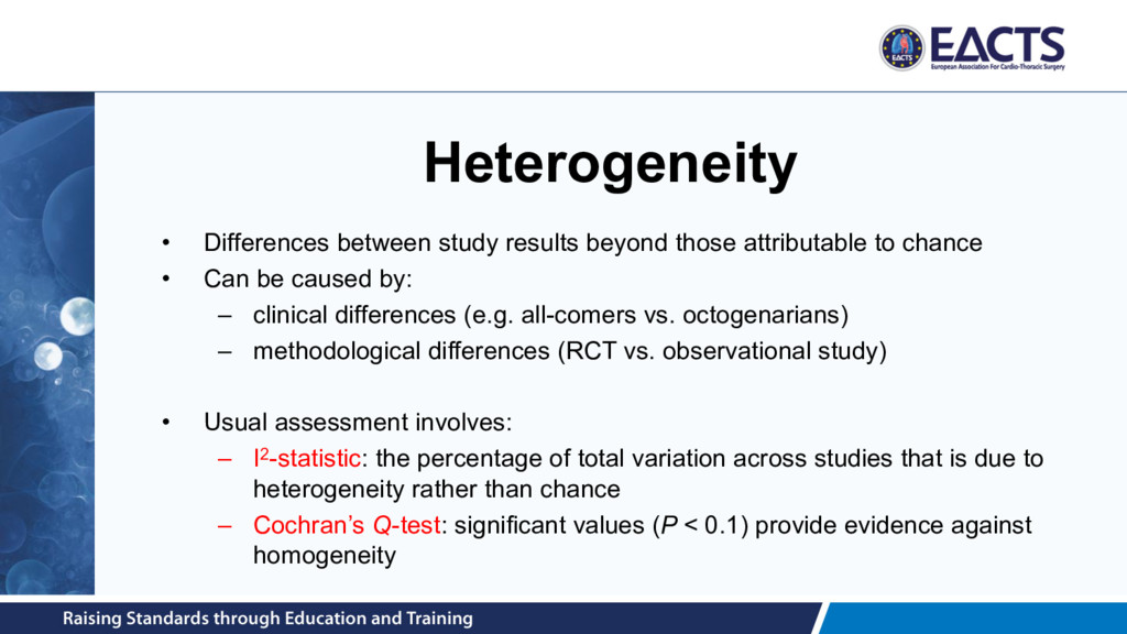
56. Heterogeneity • Differences between study results beyond those attributable to chance • Can be caused by: – clinical differences (e.g. all-comers vs. octogenarians) – methodological differences (RCT vs. observational study) • Usual assessment involves: – I2-statistic: the percentage of total variation across studies that is due to heterogeneity rather than chance – Cochran’s Q-test: significant values (P < 0.1) provide evidence against homogeneity
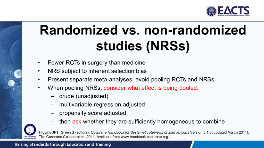
57. Randomized vs. non-randomized studies (NRSs) • Fewer RCTs in surgery than medicine • NRS subject to inherent selection bias • Present separate meta-analyses; avoid pooling RCTs and NRSs • When pooling NRSs, consider what effect is being pooled: – crude (unadjusted) – multivariable regression adjusted – propensity score adjusted – then ask whether they are sufficiently homogeneous to combine Higgins JPT, Green S (editors). Cochrane Handbook for Systematic Reviews of Interventions Version 5.1.0 [updated March 2011]. The Cochrane Collaboration, 2011. Available from www.handbook.cochrane.org.
58. Reporting
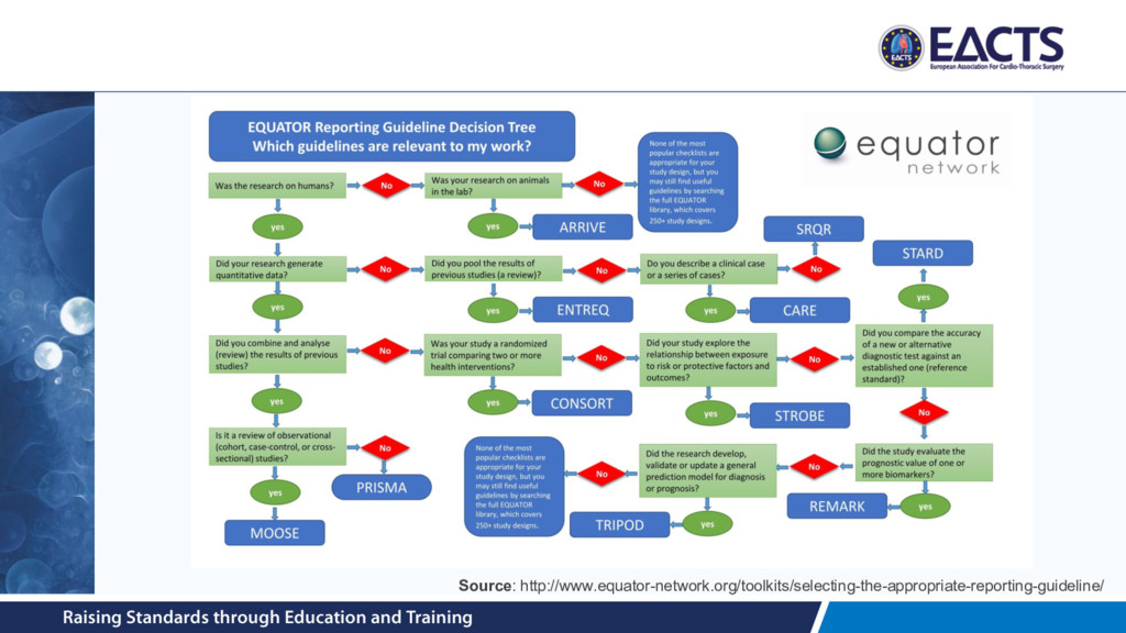
59. Reporting • Exists continued need to improve the reliability and value of published health research literature • To encourage this there are several transparent and accurate reporting guidelines available • Checklists often required by journals at time of submission http://www.equator-network.org
60. Source: http://www.equator-network.org/toolkits/selecting-the-appropriate-reporting-guideline/
62. Thank you for listening Any questions? New series of statistical “primers” forthcoming in the EJCTS and ICVTS Acknowledgements Dr. Stuart J. Head (L) Dr. Stuart W. Grant (R)