modelling of multivariate longitudinal and time-to-event data Graeme L. Hickey1, Pete Philipson2, Andrea Jorgensen1, Ruwanthi-Kolamunnage-Dona1 1Department of Biostatistics, University of Liverpool, UK 2Mathematics, Physics and Electrical Engineering, University of Northumbria, UK [email protected] Funded by Grant MR/M013227/1 14th March 2018 GL. Hickey Joint modelling of multivariate data 1 / 55
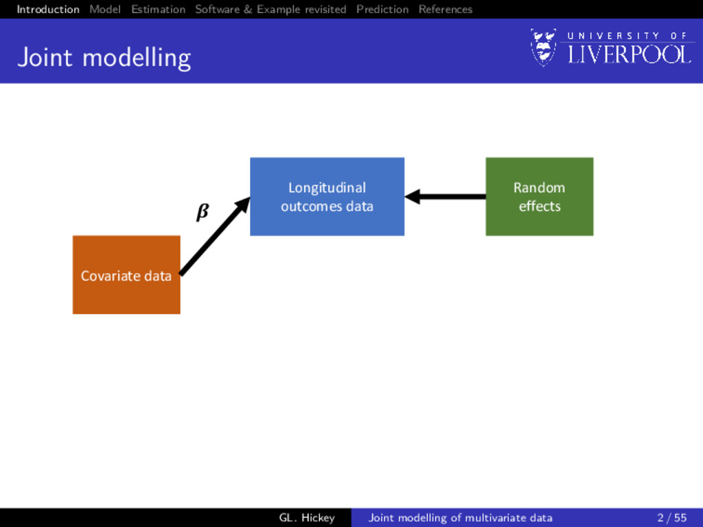
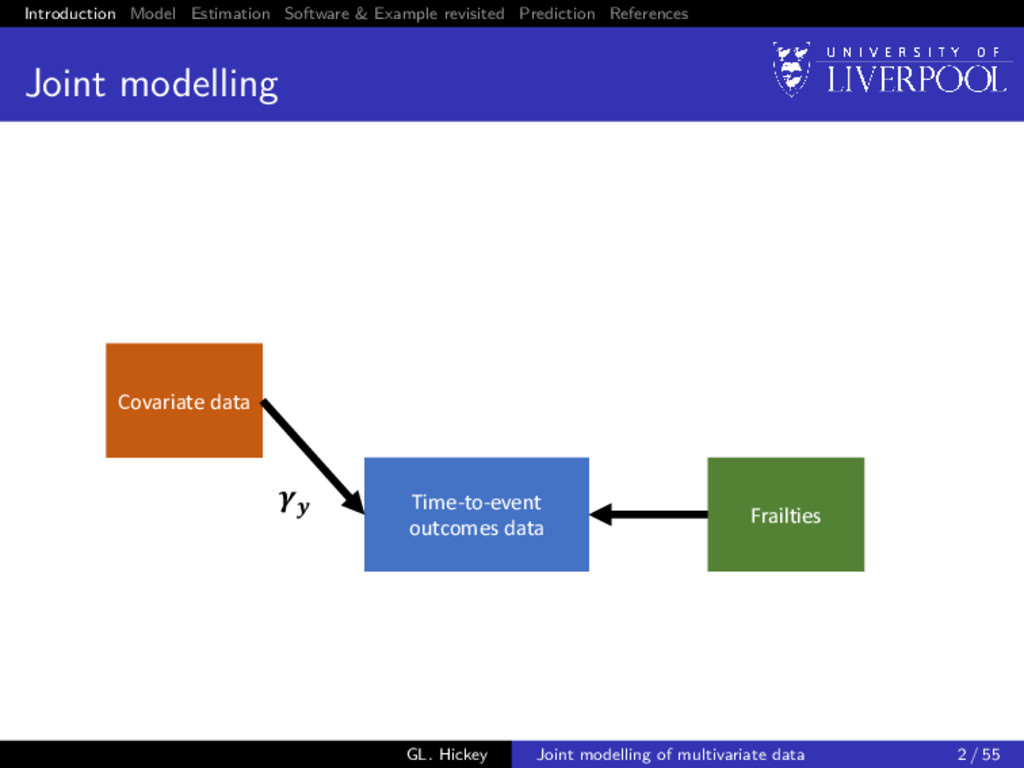
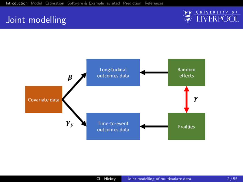
modelling Covariate data Time-to-event outcomes data Frailties Longitudinal outcomes data Random effects GL. Hickey Joint modelling of multivariate data 2 / 55
modelling Covariate data Time-to-event outcomes data Frailties Longitudinal outcomes data Random effects GL. Hickey Joint modelling of multivariate data 2 / 55
use a joint model? Interest lies with adjustment of inferences about longitudinal measurements for possibly outcome-dependent drop-out adjustment of inferences about the time-to-event distribution conditional on intermediate and/or error prone longitudinal measurements the joint evolution of the measurement and event time processes biomarker surrogacy dynamic prediction GL. Hickey Joint modelling of multivariate data 3 / 55
for multivariate joint models Clinical studies often repeatedly measure multiple biomarkers or other measurements and an event time Research has predominantly focused on a single event time and single measurement outcome Ignoring correlation leads to bias and reduced efficiency in estimation Harnessing all available information in a single model is advantageous and should lead to improved model predictions GL. Hickey Joint modelling of multivariate data 4 / 55
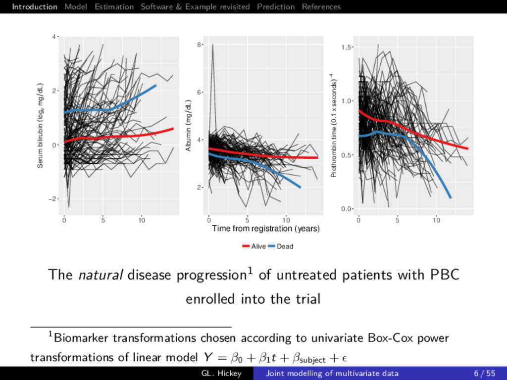
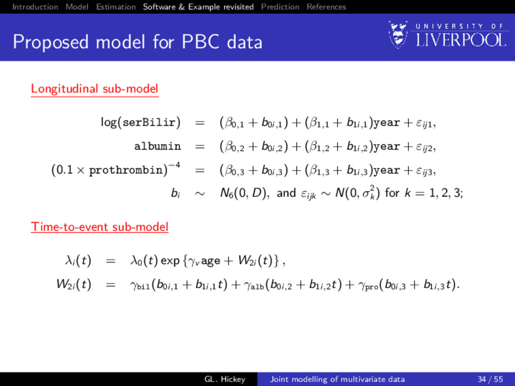
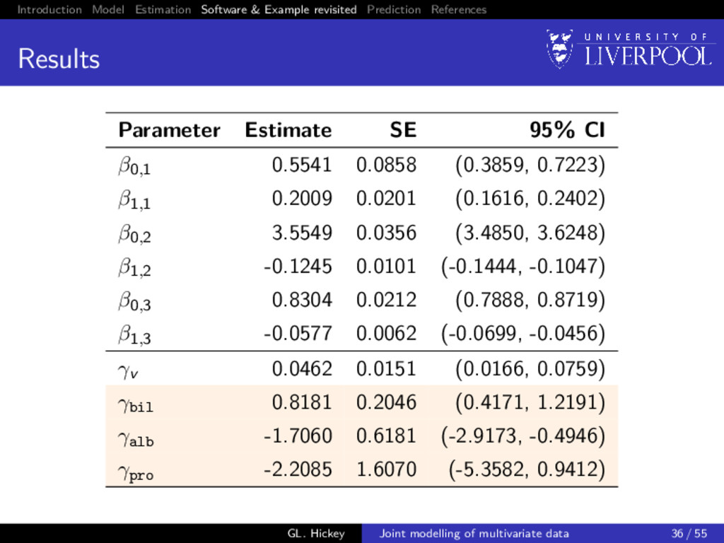
example Primary biliary cirrhosis (PBC) is a chronic liver disease characterized by inflammatory destruction of the small bile ducts, which eventually leads to cirrhosis of the liver and death Consider a subset of 154 patients randomized to placebo treatment from Mayo Clinic trial (Murtaugh et al. 1994) Multiple biomarkers repeatedly measured at intermittent times, of which we consider 3 clinically relevant ones: 1 serum bilirunbin (mg/dl) 2 serum albumin (mg/dl) 3 prothrombin time (seconds) GL. Hickey Joint modelling of multivariate data 5 / 55
time (0.1 x seconds)−4 Albumin (mg dL) Serum bilirubin (loge mg dL) 0 5 10 0 5 10 0 5 10 0.0 0.5 1.0 1.5 2 4 6 8 −2 0 2 4 Time from registration (years) Alive Dead The natural disease progression1 of untreated patients with PBC enrolled into the trial 1Biomarker transformations chosen according to univariate Box-Cox power transformations of linear model Y = β0 + β1 t + βsubject + GL. Hickey Joint modelling of multivariate data 6 / 55
of the rest of the talk Model development Extend existing models for multivariate data and develop practical fitting strategies GL. Hickey Joint modelling of multivariate data 8 / 55
of the rest of the talk Model development Extend existing models for multivariate data and develop practical fitting strategies Dynamic prediction Extend modelling framework for dynamic prediction purposes and explore utility of multiple longitudinal outcomes GL. Hickey Joint modelling of multivariate data 8 / 55
of the rest of the talk Model development Extend existing models for multivariate data and develop practical fitting strategies Dynamic prediction Extend modelling framework for dynamic prediction purposes and explore utility of multiple longitudinal outcomes Software development Present an –package that implements these methods GL. Hickey Joint modelling of multivariate data 8 / 55
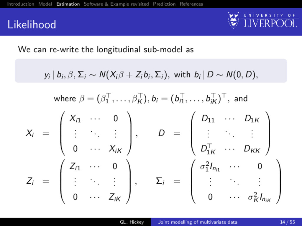
For each subject i = 1, . . . , n, we observe yi = (yi1 , . . . , yiK ) is a K-variate continuous outcome vector, where each yik denotes an (nik × 1)-vector of observed longitudinal measurements for the k-th outcome type: yik = (yi1k, . . . , yinik k) Observation times tijk for j = 1, . . . , nik, which can differ between subjects and outcomes (Ti , δi ), where Ti = min(T∗ i , Ci ), where T∗ i is the true event time, Ci corresponds to a potential right-censoring time, and δi is the failure indicator equal to 1 if the failure is observed (T∗ i ≤ Ci ) and 0 otherwise GL. Hickey Joint modelling of multivariate data 9 / 55
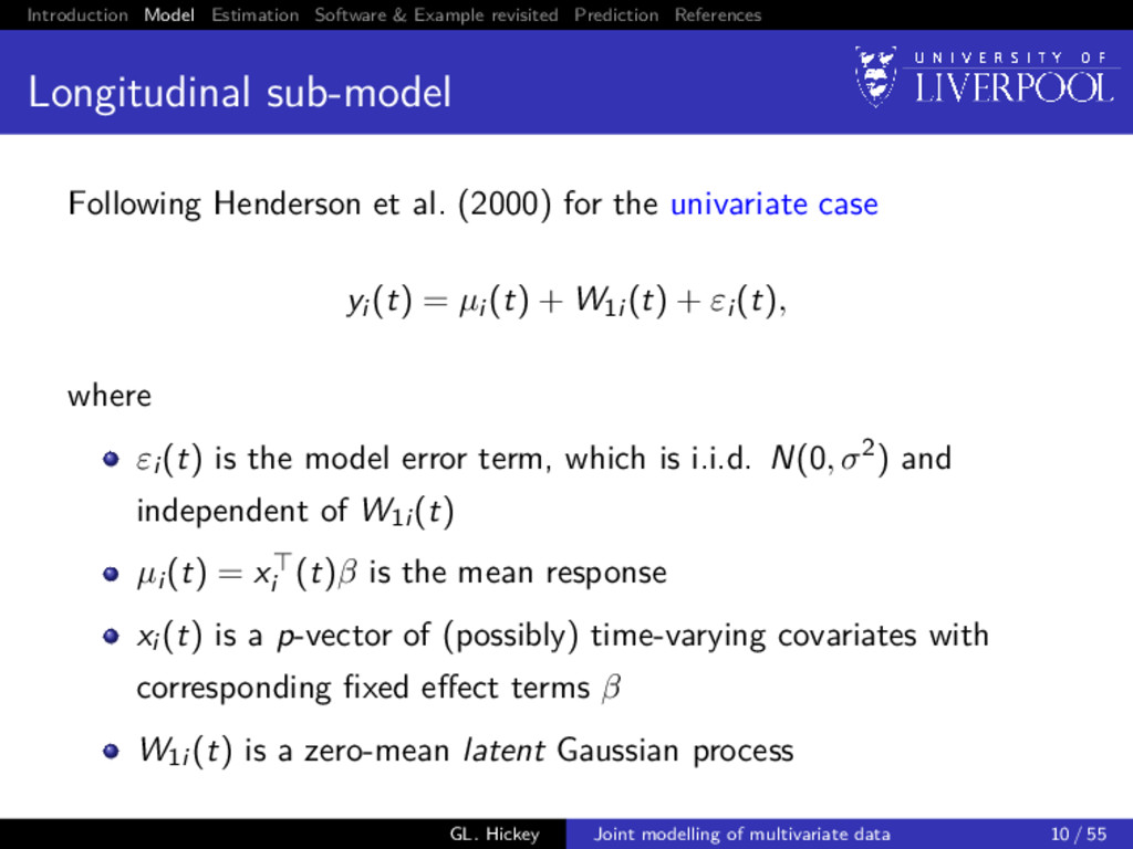
sub-model Following Henderson et al. (2000) for the univariate case yi (t) = µi (t) + W1i (t) + εi (t), where εi (t) is the model error term, which is i.i.d. N(0, σ2) and independent of W1i (t) µi (t) = xi (t)β is the mean response xi (t) is a p-vector of (possibly) time-varying covariates with corresponding fixed effect terms β W1i (t) is a zero-mean latent Gaussian process GL. Hickey Joint modelling of multivariate data 10 / 55
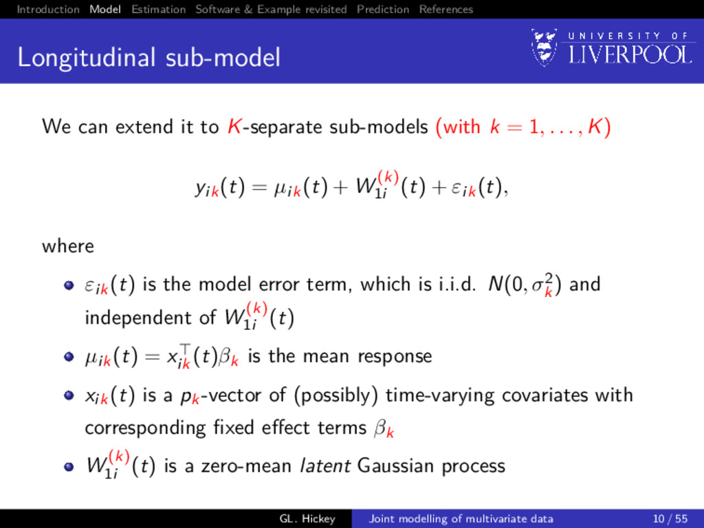
sub-model We can extend it to K-separate sub-models (with k = 1, . . . , K) yik(t) = µik(t) + W (k) 1i (t) + εik(t), where εik(t) is the model error term, which is i.i.d. N(0, σ2 k ) and independent of W (k) 1i (t) µik(t) = xik (t)βk is the mean response xik(t) is a pk-vector of (possibly) time-varying covariates with corresponding fixed effect terms βk W (k) 1i (t) is a zero-mean latent Gaussian process GL. Hickey Joint modelling of multivariate data 10 / 55
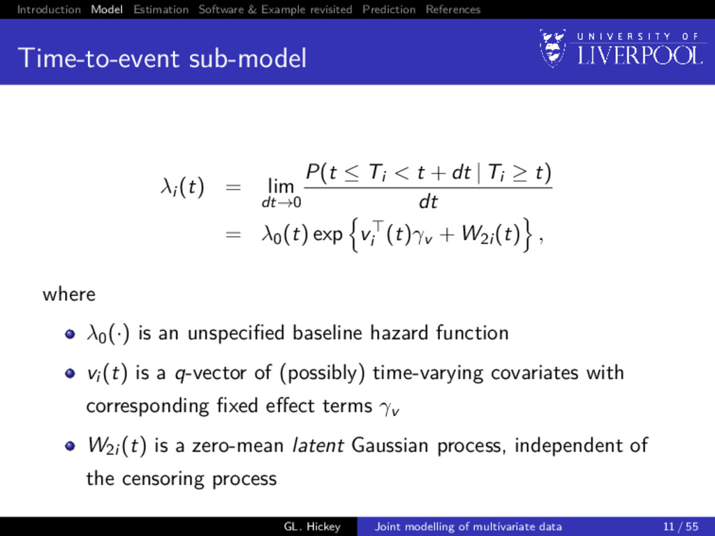
sub-model λi (t) = lim dt→0 P(t ≤ Ti < t + dt | Ti ≥ t) dt = λ0(t) exp vi (t)γv + W2i (t) , where λ0(·) is an unspecified baseline hazard function vi (t) is a q-vector of (possibly) time-varying covariates with corresponding fixed effect terms γv W2i (t) is a zero-mean latent Gaussian process, independent of the censoring process GL. Hickey Joint modelling of multivariate data 11 / 55
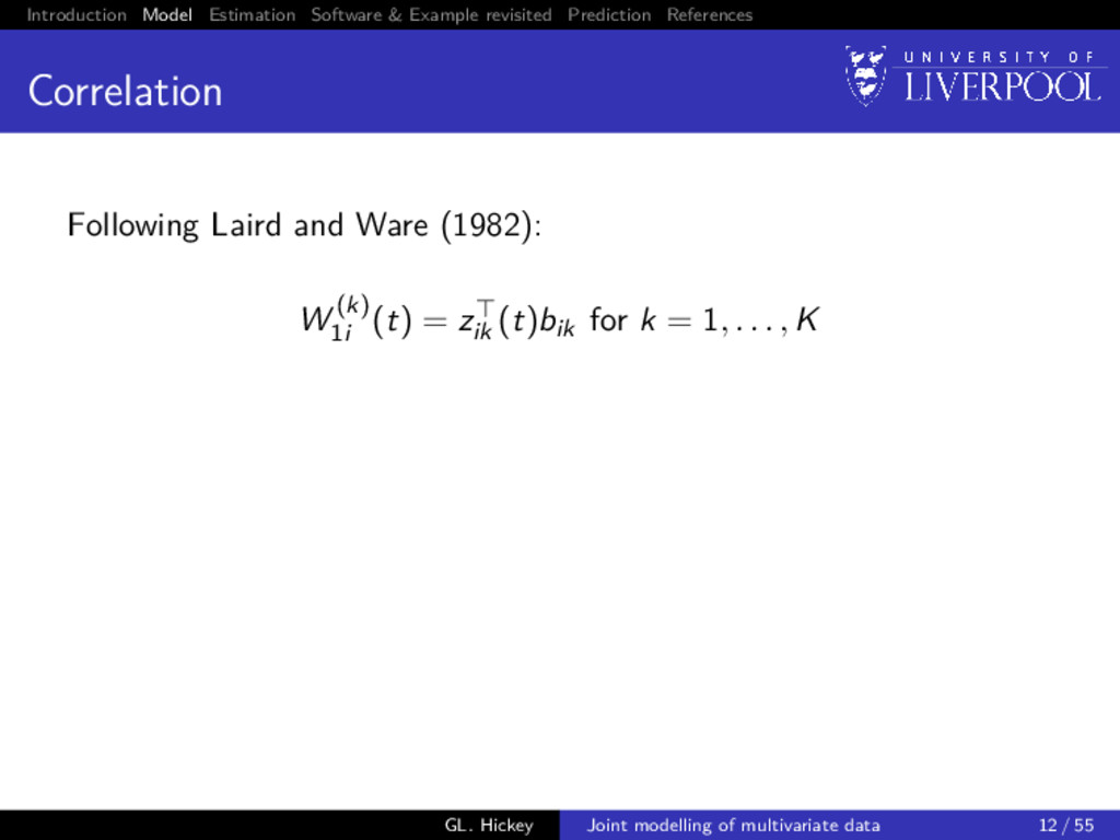
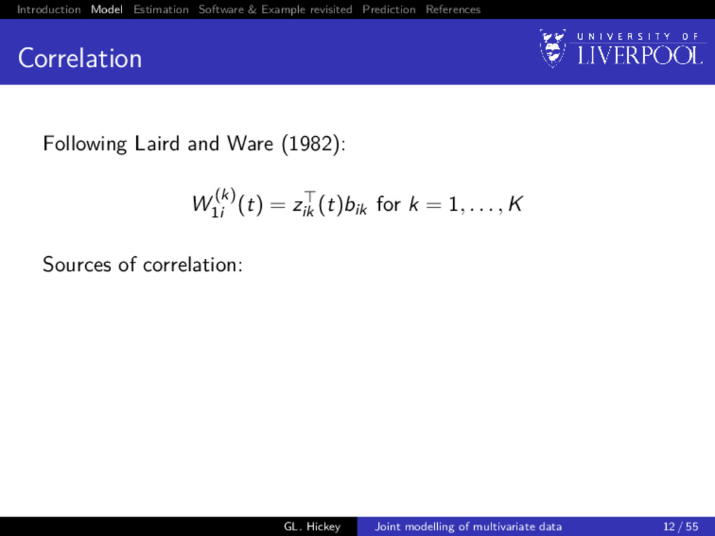
Following Laird and Ware (1982): W (k) 1i (t) = zik (t)bik for k = 1, . . . , K Sources of correlation: GL. Hickey Joint modelling of multivariate data 12 / 55
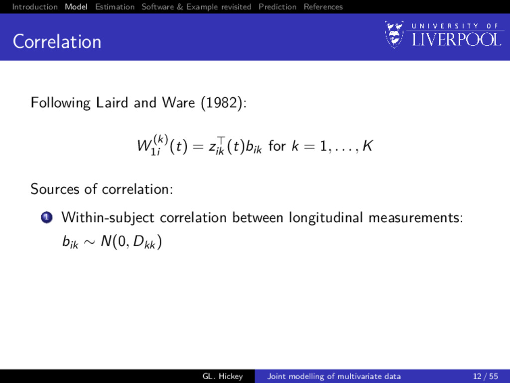
Following Laird and Ware (1982): W (k) 1i (t) = zik (t)bik for k = 1, . . . , K Sources of correlation: 1 Within-subject correlation between longitudinal measurements: bik ∼ N(0, Dkk) GL. Hickey Joint modelling of multivariate data 12 / 55
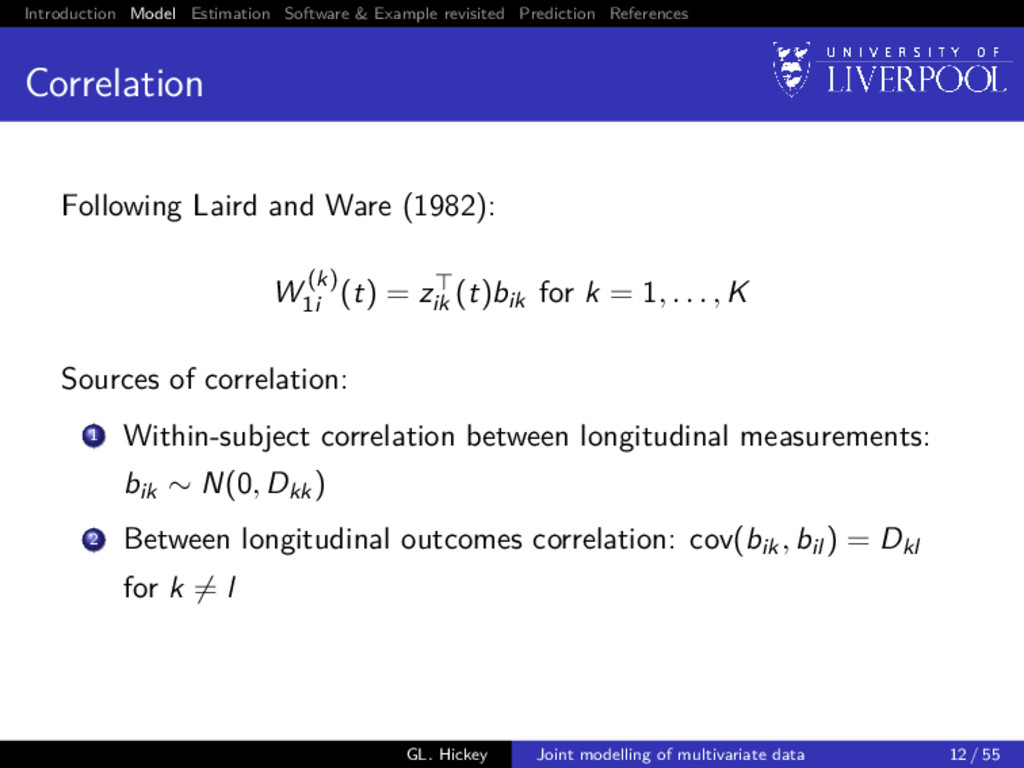
Following Laird and Ware (1982): W (k) 1i (t) = zik (t)bik for k = 1, . . . , K Sources of correlation: 1 Within-subject correlation between longitudinal measurements: bik ∼ N(0, Dkk) 2 Between longitudinal outcomes correlation: cov(bik, bil ) = Dkl for k = l GL. Hickey Joint modelling of multivariate data 12 / 55
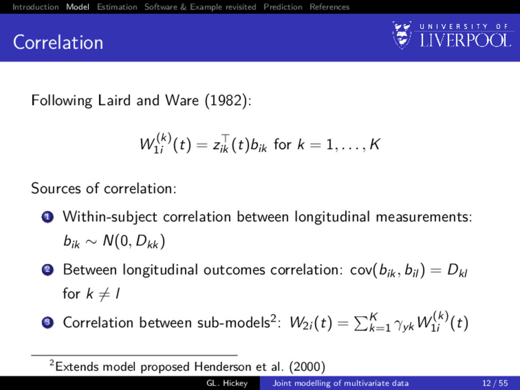
Following Laird and Ware (1982): W (k) 1i (t) = zik (t)bik for k = 1, . . . , K Sources of correlation: 1 Within-subject correlation between longitudinal measurements: bik ∼ N(0, Dkk) 2 Between longitudinal outcomes correlation: cov(bik, bil ) = Dkl for k = l 3 Correlation between sub-models2: W2i (t) = K k=1 γykW (k) 1i (t) 2Extends model proposed Henderson et al. (2000) GL. Hickey Joint modelling of multivariate data 12 / 55
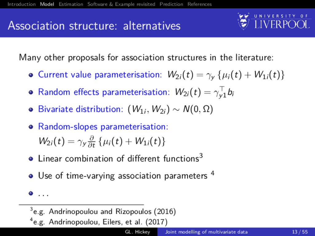
structure: alternatives Many other proposals for association structures in the literature: Current value parameterisation: W2i (t) = γy {µi (t) + W1i (t)} Random effects parameterisation: W2i (t) = γy1 bi Bivariate distribution: (W1i , W2i ) ∼ N(0, Ω) Random-slopes parameterisation: W2i (t) = γy ∂ ∂t {µi (t) + W1i (t)} Linear combination of different functions3 Use of time-varying association parameters 4 . . . 3e.g. Andrinopoulou and Rizopoulos (2016) 4e.g. Andrinopoulou, Eilers, et al. (2017) GL. Hickey Joint modelling of multivariate data 13 / 55
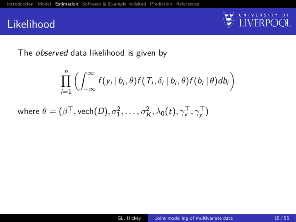
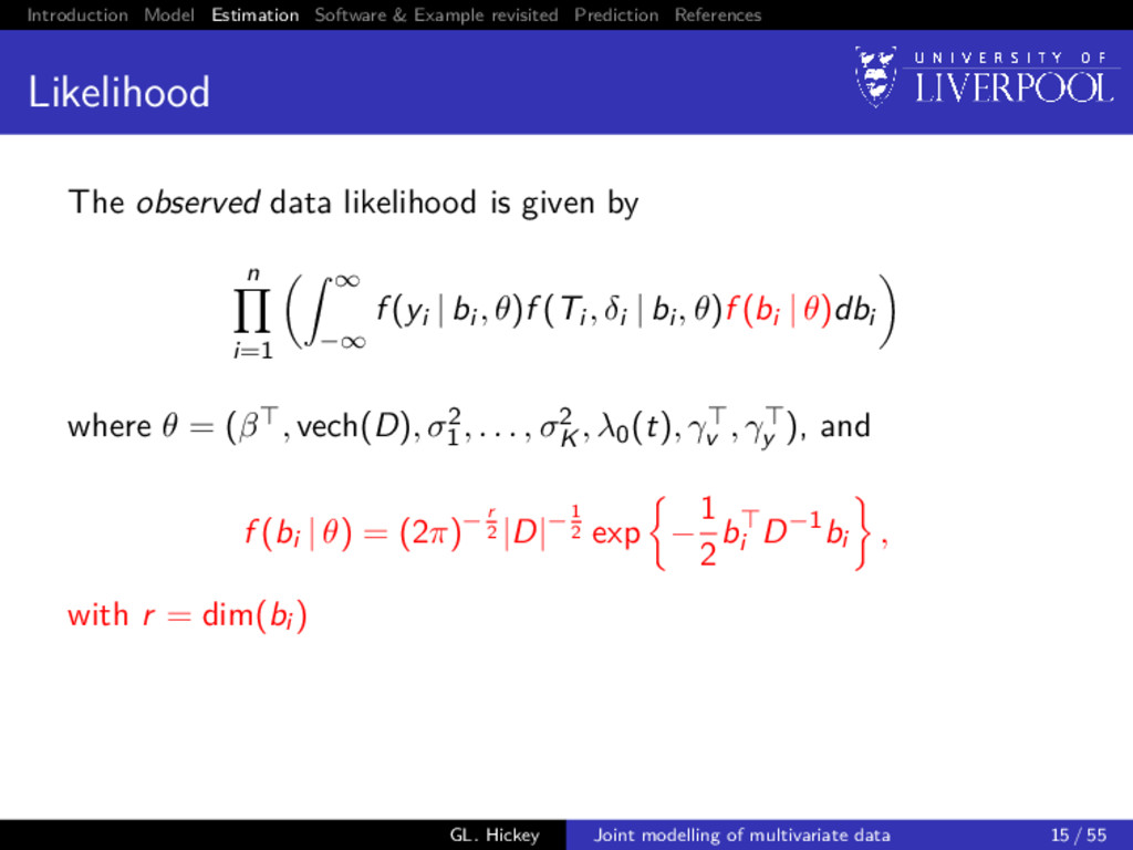
The observed data likelihood is given by n i=1 ∞ −∞ f (yi | bi , θ)f (Ti , δi | bi , θ)f (bi | θ)dbi where θ = (β , vech(D), σ2 1 , . . . , σ2 K , λ0(t), γv , γy ) GL. Hickey Joint modelling of multivariate data 15 / 55
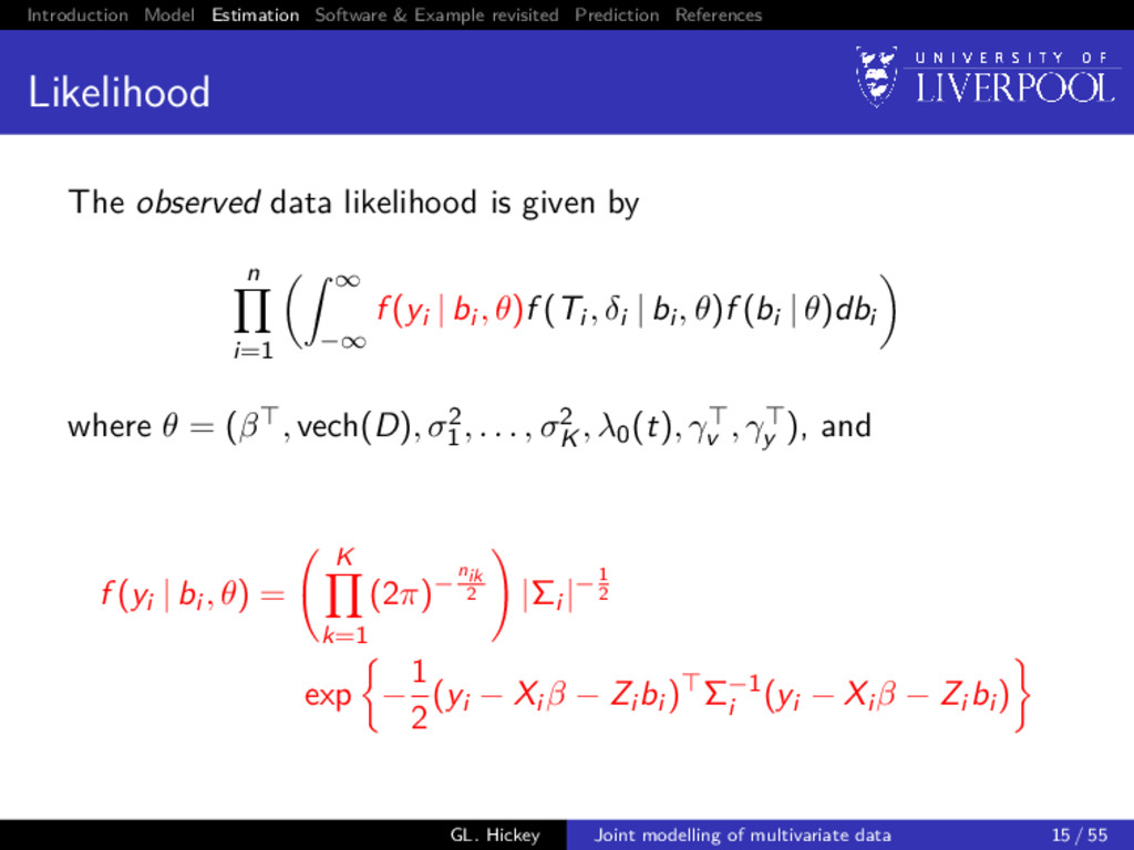
The observed data likelihood is given by n i=1 ∞ −∞ f (yi | bi , θ)f (Ti , δi | bi , θ)f (bi | θ)dbi where θ = (β , vech(D), σ2 1 , . . . , σ2 K , λ0(t), γv , γy ), and f (yi | bi , θ) = K k=1 (2π)−nik 2 |Σi |−1 2 exp − 1 2 (yi − Xi β − Zi bi ) Σ−1 i (yi − Xi β − Zi bi ) GL. Hickey Joint modelling of multivariate data 15 / 55
The observed data likelihood is given by n i=1 ∞ −∞ f (yi | bi , θ)f (Ti , δi | bi , θ)f (bi | θ)dbi where θ = (β , vech(D), σ2 1 , . . . , σ2 K , λ0(t), γv , γy ), and f (Ti , δi | bi ; θ) = λ0(Ti ) exp vi γv + W2i (Ti , bi ) δi exp − Ti 0 λ0(u) exp vi γv + W2i (u, bi ) du GL. Hickey Joint modelling of multivariate data 15 / 55
The observed data likelihood is given by n i=1 ∞ −∞ f (yi | bi , θ)f (Ti , δi | bi , θ)f (bi | θ)dbi where θ = (β , vech(D), σ2 1 , . . . , σ2 K , λ0(t), γv , γy ), and f (bi | θ) = (2π)− r 2 |D|−1 2 exp − 1 2 bi D−1bi , with r = dim(bi ) GL. Hickey Joint modelling of multivariate data 15 / 55
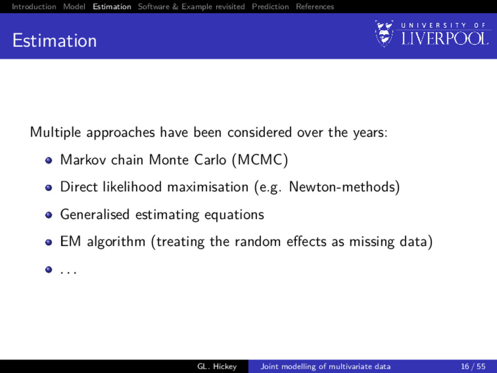
Multiple approaches have been considered over the years: Markov chain Monte Carlo (MCMC) Direct likelihood maximisation (e.g. Newton-methods) Generalised estimating equations EM algorithm (treating the random effects as missing data) . . . GL. Hickey Joint modelling of multivariate data 16 / 55
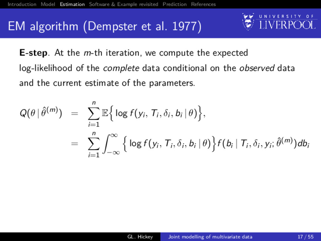
algorithm (Dempster et al. 1977) E-step. At the m-th iteration, we compute the expected log-likelihood of the complete data conditional on the observed data and the current estimate of the parameters. Q(θ | ˆ θ(m)) = n i=1 E log f (yi , Ti , δi , bi | θ) , = n i=1 ∞ −∞ log f (yi , Ti , δi , bi | θ) f (bi | Ti , δi , yi ; ˆ θ(m))dbi GL. Hickey Joint modelling of multivariate data 17 / 55
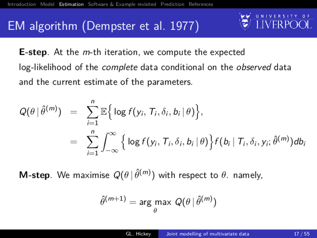
algorithm (Dempster et al. 1977) E-step. At the m-th iteration, we compute the expected log-likelihood of the complete data conditional on the observed data and the current estimate of the parameters. Q(θ | ˆ θ(m)) = n i=1 E log f (yi , Ti , δi , bi | θ) , = n i=1 ∞ −∞ log f (yi , Ti , δi , bi | θ) f (bi | Ti , δi , yi ; ˆ θ(m))dbi M-step. We maximise Q(θ | ˆ θ(m)) with respect to θ. namely, ˆ θ(m+1) = arg max θ Q(θ | ˆ θ(m)) GL. Hickey Joint modelling of multivariate data 17 / 55
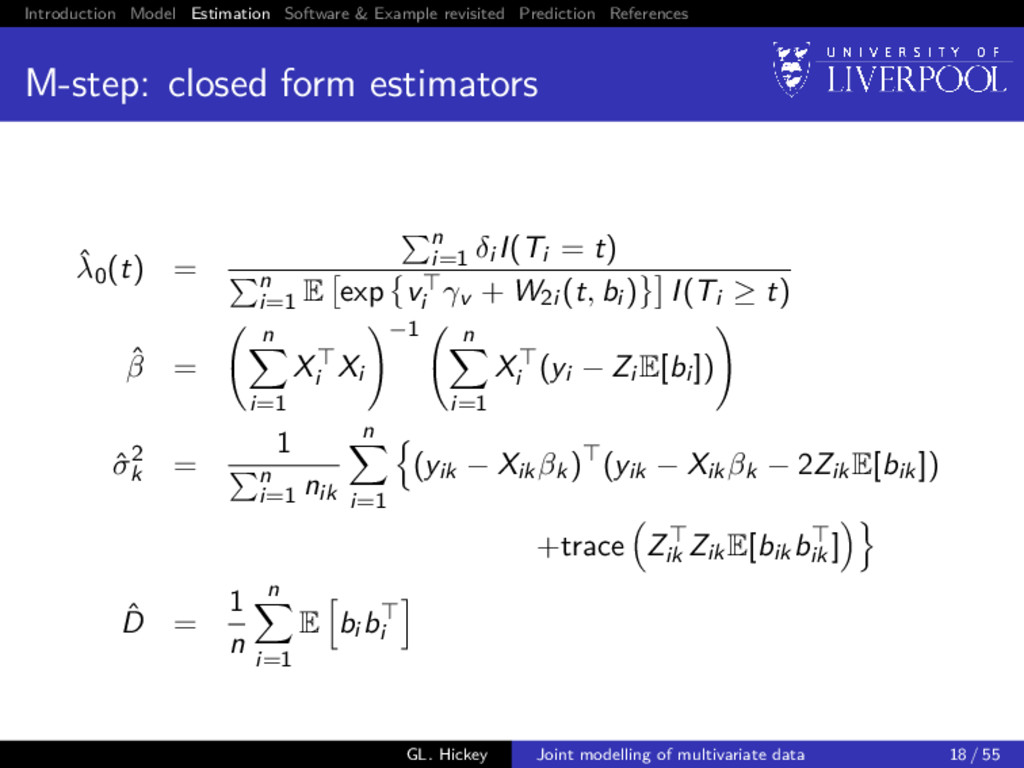
closed form estimators ˆ λ0(t) = n i=1 δi I(Ti = t) n i=1 E exp vi γv + W2i (t, bi ) I(Ti ≥ t) ˆ β = n i=1 Xi Xi −1 n i=1 Xi (yi − Zi E[bi ]) ˆ σ2 k = 1 n i=1 nik n i=1 (yik − Xikβk) (yik − Xikβk − 2ZikE[bik]) +trace Zik ZikE[bikbik ] ˆ D = 1 n n i=1 E bi bi GL. Hickey Joint modelling of multivariate data 18 / 55
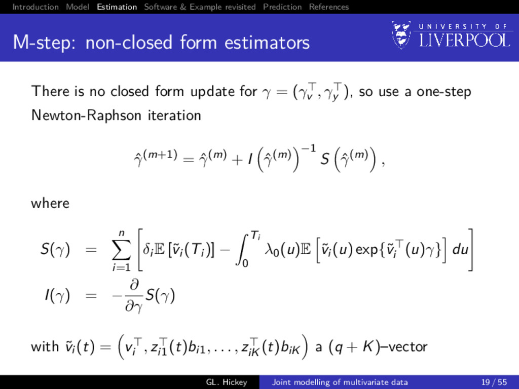
non-closed form estimators There is no closed form update for γ = (γv , γy ), so use a one-step Newton-Raphson iteration ˆ γ(m+1) = ˆ γ(m) + I ˆ γ(m) −1 S ˆ γ(m) , where S(γ) = n i=1 δi E [˜ vi (Ti )] − Ti 0 λ0(u)E ˜ vi (u) exp{˜ vi (u)γ} du I(γ) = − ∂ ∂γ S(γ) with ˜ vi (t) = vi , zi1 (t)bi1, . . . , ziK (t)biK a (q + K)–vector GL. Hickey Joint modelling of multivariate data 19 / 55
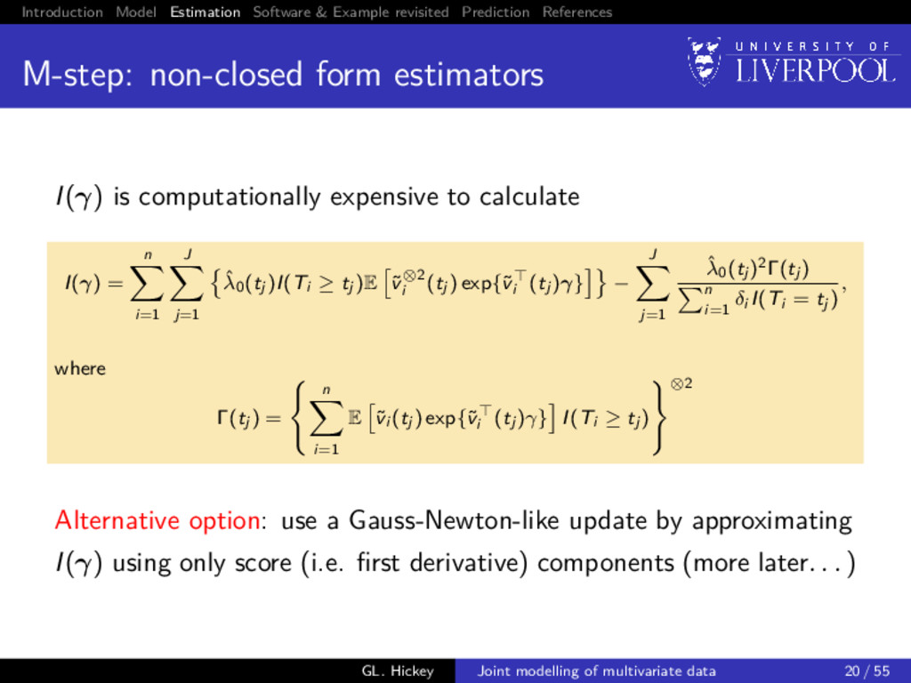
non-closed form estimators I(γ) is computationally expensive to calculate I(γ) = n i=1 J j=1 ˆ λ0(tj )I(Ti ≥ tj )E ˜ v⊗2 i (tj ) exp{˜ vi (tj )γ} − J j=1 ˆ λ0(tj )2Γ(tj ) n i=1 δi I(Ti = tj ) , where Γ(tj ) = n i=1 E ˜ vi (tj ) exp{˜ vi (tj )γ} I(Ti ≥ tj ) ⊗2 Alternative option: use a Gauss-Newton-like update by approximating I(γ) using only score (i.e. first derivative) components (more later. . . ) GL. Hickey Joint modelling of multivariate data 20 / 55
algorithm E-step requires calculating several multidimensional integrals of form E h(bi ) | Ti , δi , yi ; ˆ θ Gauss-quadrature can be slow if dim(bi ) is large ⇒ might not scale well as K increases (Recall: EM algorithm has first-order convergence) Instead, we use the Monte Carlo Expectation-Maximization (MCEM)5 M-step updates remain the same 5Wei and Tanner (1990) GL. Hickey Joint modelling of multivariate data 21 / 55
Carlo E-step Conventional EM algorithm: use quadrature to compute E h(bi ) | Ti , δi , yi ; ˆ θ = ∞ −∞ h(bi )f (bi | yi ; ˆ θ)f (Ti , δi | bi ; ˆ θ)dbi ∞ −∞ f (bi | yi ; ˆ θ)f (Ti , δi | bi ; ˆ θ)dbi , where h(·) = any known fuction, bi | yi , θ ∼ N Ai Zi Σ−1 i (yi − Xi β) , Ai , and Ai = Zi Σ−1 i Zi + D−1 −1 GL. Hickey Joint modelling of multivariate data 22 / 55
Carlo E-step MCEM algorithm E-step: use Monte Carlo integration to compute E h(bi ) | Ti , δi , yi ; ˆ θ ≈ 1 N N d=1 h b(d) i f Ti , δi | b(d) i ; ˆ θ 1 N N d=1 f Ti , δi | b(d) i ; ˆ θ where h(·) = any known fuction, bi | yi , θ ∼ N Ai Zi Σ−1 i (yi − Xi β) , Ai , and Ai = Zi Σ−1 i Zi + D−1 −1 b(1) i , b(2) i , . . . , b(N) i ∼ bi | yi , θ a Monte Carlo draw GL. Hickey Joint modelling of multivariate data 22 / 55
of MC integration We consider 3 different flavours of Monte Carlo (MC) integration: 1 Ordinary MC 2 Variance reduction MC Antithetic variates 3 Quasi-MC Sobol sequence Halton sequence GL. Hickey Joint modelling of multivariate data 23 / 55
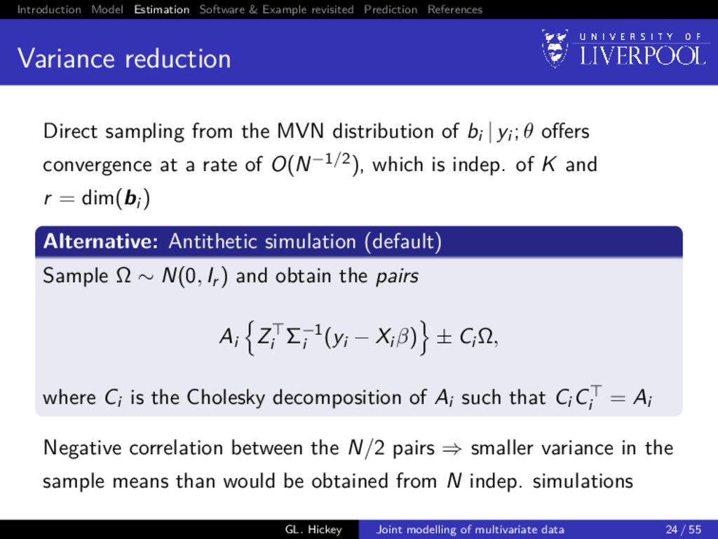
reduction Direct sampling from the MVN distribution of bi | yi ; θ offers convergence at a rate of O(N−1/2), which is indep. of K and r = dim(bi ) Alternative: Antithetic simulation (default) Sample Ω ∼ N(0, Ir ) and obtain the pairs Ai Zi Σ−1 i (yi − Xi β) ± Ci Ω, where Ci is the Cholesky decomposition of Ai such that Ci Ci = Ai Negative correlation between the N/2 pairs ⇒ smaller variance in the sample means than would be obtained from N indep. simulations GL. Hickey Joint modelling of multivariate data 24 / 55
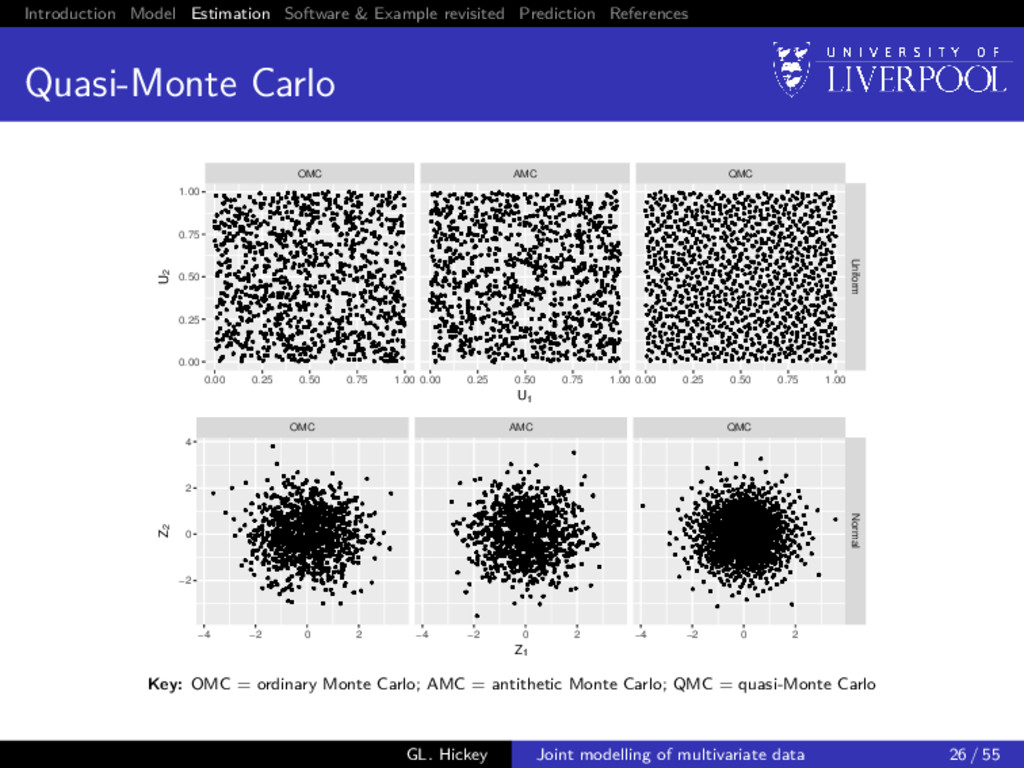
Carlo Replaces the (pseudo-)random sequence by a deterministic one Sobol sequence Halton sequence . . . Quasi-random sequences yield smaller errors than standard MC integration methods Convergence is O (logN)r N Early results promising + on-going research via intensive simulation . . . GL. Hickey Joint modelling of multivariate data 25 / 55
In standard EM, convergence usually declared at (m + 1)-th iteration if one of the following criteria satisfied Relative change: ∆(m+1) rel = max |ˆ θ(m+1)−ˆ θ(m)| |ˆ θ(m)|+ 1 < 0 Absolute change: ∆(m+1) abs = max |ˆ θ(m+1) − ˆ θ(m)| < 2 for some choice of 0, 1, and 2 GL. Hickey Joint modelling of multivariate data 27 / 55
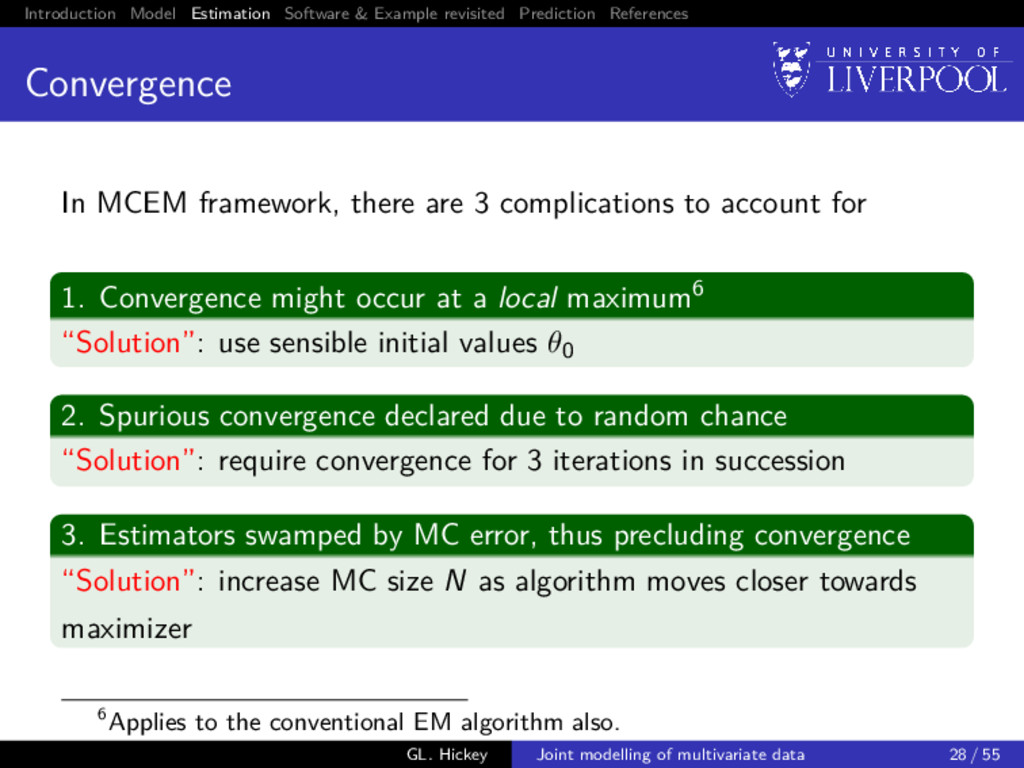
In MCEM framework, there are 3 complications to account for 1. Convergence might occur at a local maximum6 “Solution”: use sensible initial values θ0 6Applies to the conventional EM algorithm also. GL. Hickey Joint modelling of multivariate data 28 / 55
In MCEM framework, there are 3 complications to account for 1. Convergence might occur at a local maximum6 “Solution”: use sensible initial values θ0 2. Spurious convergence declared due to random chance “Solution”: require convergence for 3 iterations in succession 6Applies to the conventional EM algorithm also. GL. Hickey Joint modelling of multivariate data 28 / 55
In MCEM framework, there are 3 complications to account for 1. Convergence might occur at a local maximum6 “Solution”: use sensible initial values θ0 2. Spurious convergence declared due to random chance “Solution”: require convergence for 3 iterations in succession 3. Estimators swamped by MC error, thus precluding convergence “Solution”: increase MC size N as algorithm moves closer towards maximizer 6Applies to the conventional EM algorithm also. GL. Hickey Joint modelling of multivariate data 28 / 55
values Multivariate longitudinal sub-model Ordinary EM-algorithm: E-step is closed-form, so can be made quick Time-to-event sub-model If balanced (i.e. tijk = tij ∀k), then fit a two-stage model using the BLUPs for the MV-LMM (above) using (Anderson-Gill counting process) Cox model If unbalanced, γy = 0 and γv estimated using a standard Cox PH model Alternatively, specify them manually from expert knowledge GL. Hickey Joint modelling of multivariate data 29 / 55
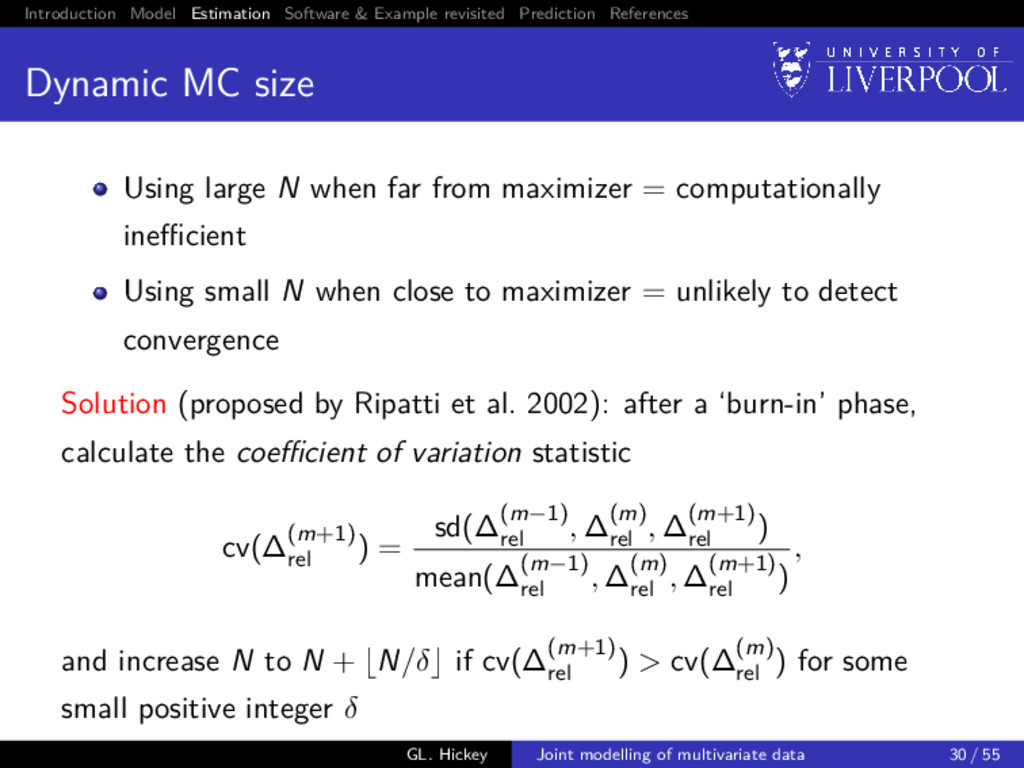
MC size Using large N when far from maximizer = computationally inefficient Using small N when close to maximizer = unlikely to detect convergence Solution (proposed by Ripatti et al. 2002): after a ‘burn-in’ phase, calculate the coefficient of variation statistic cv(∆(m+1) rel ) = sd(∆(m−1) rel , ∆(m) rel , ∆(m+1) rel ) mean(∆(m−1) rel , ∆(m) rel , ∆(m+1) rel ) , and increase N to N + N/δ if cv(∆(m+1) rel ) > cv(∆(m) rel ) for some small positive integer δ GL. Hickey Joint modelling of multivariate data 30 / 55
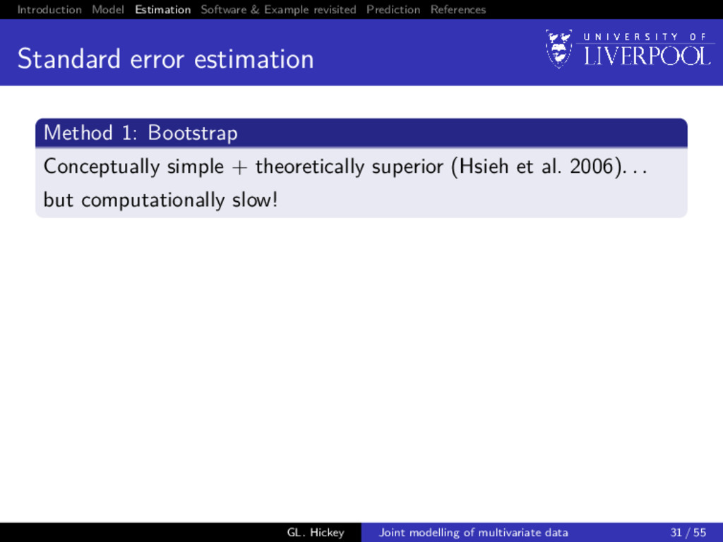
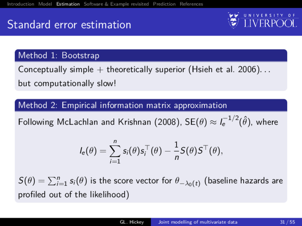
error estimation Method 1: Bootstrap Conceptually simple + theoretically superior (Hsieh et al. 2006). . . but computationally slow! Method 2: Empirical information matrix approximation Following McLachlan and Krishnan (2008), SE(θ) ≈ I−1/2 e (ˆ θ), where Ie(θ) = n i=1 si (θ)si (θ) − 1 n S(θ)S (θ), S(θ) = n i=1 si (θ) is the score vector for θ−λ0(t) (baseline hazards are profiled out of the likelihood) GL. Hickey Joint modelling of multivariate data 31 / 55
package options JMbayes: extends the existing R package (by Dimitris Rizopoulos, Erasmus MC) rstanarm: absorbs the now defunct R package rstanjm (by Sam Brilleman, Monash University) stjm: extends the existing Stata package (by Michael Crowther, University of Leicester) megenreg: similar to stjm, but can handle other models (also by Michael Crowther, University of Leicester) GL. Hickey Joint modelling of multivariate data 33 / 55
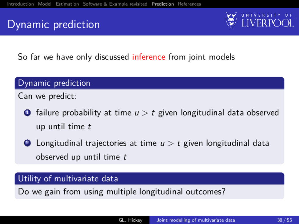
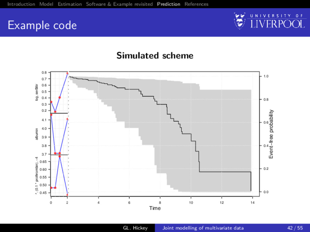
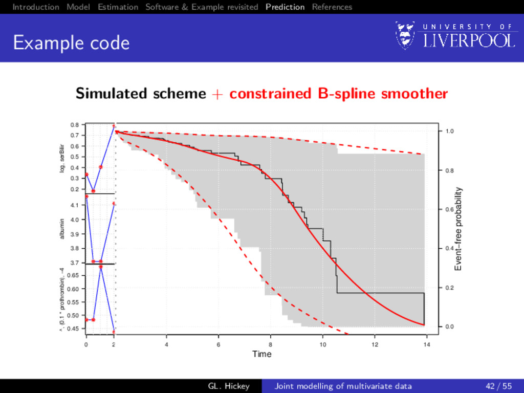
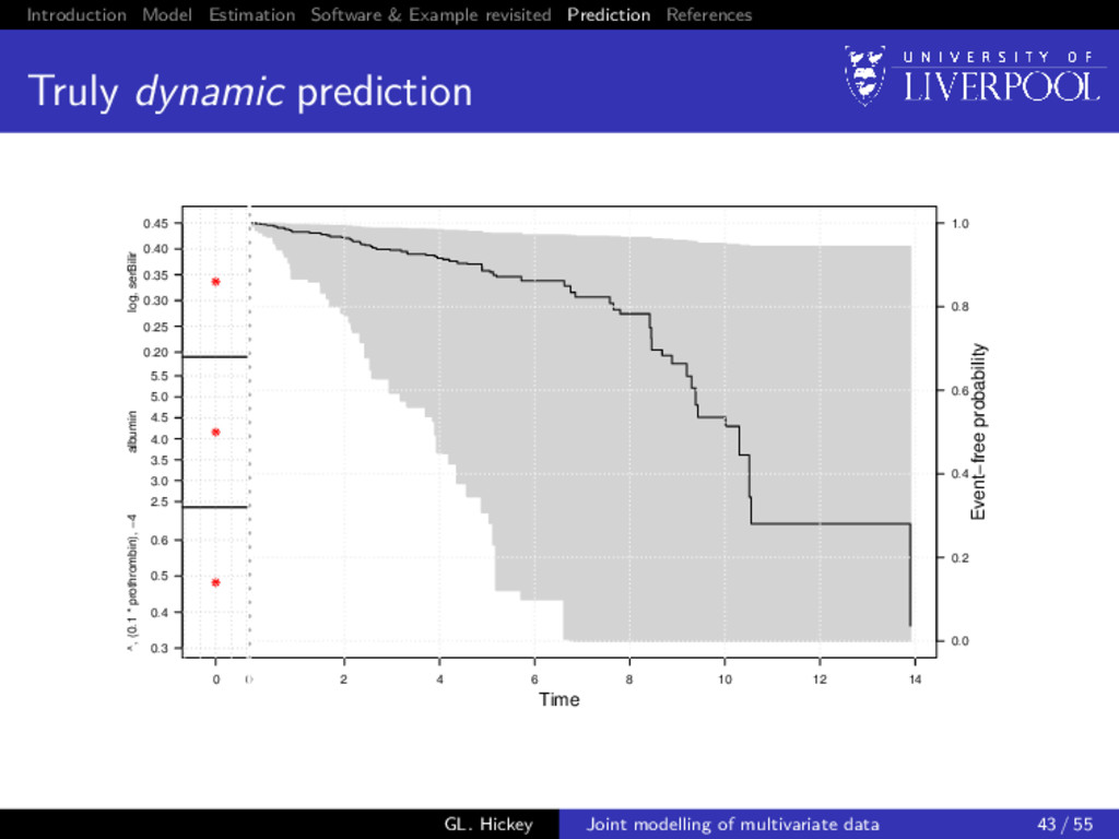
prediction So far we have only discussed inference from joint models Dynamic prediction Can we predict: 1 failure probability at time u > t given longitudinal data observed up until time t 2 Longitudinal trajectories at time u > t given longitudinal data observed up until time t Utility of multivariate data Do we gain from using multiple longitudinal outcomes? GL. Hickey Joint modelling of multivariate data 38 / 55
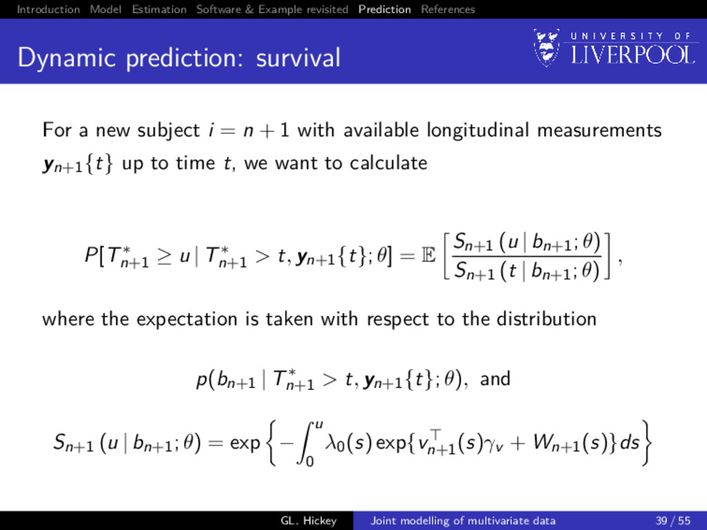
prediction: survival For a new subject i = n + 1 with available longitudinal measurements yn+1{t} up to time t, we want to calculate P[T∗ n+1 ≥ u | T∗ n+1 > t, yn+1{t}; θ] = E Sn+1 (u | bn+1; θ) Sn+1 (t | bn+1; θ) , where the expectation is taken with respect to the distribution p(bn+1 | T∗ n+1 > t, yn+1{t}; θ), and Sn+1 (u | bn+1; θ) = exp − u 0 λ0(s) exp{vn+1 (s)γv + Wn+1(s)}ds GL. Hickey Joint modelling of multivariate data 39 / 55
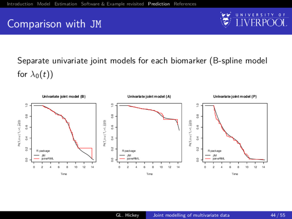
with JM Separate univariate joint models for each biomarker (B-spline model for λ0(t)) 0 2 4 6 8 10 12 14 0.0 0.2 0.4 0.6 0.8 1.0 Univariate joint model {B} Time Pr(Ti ≥ u | Ti > t, y ~ i (t)) R package JM joineRML 0 2 4 6 8 10 12 14 0.0 0.2 0.4 0.6 0.8 1.0 Univariate joint model {A} Time Pr(Ti ≥ u | Ti > t, y ~ i (t)) R package JM joineRML 0 2 4 6 8 10 12 14 0.0 0.2 0.4 0.6 0.8 1.0 Univariate joint model {P} Time Pr(Ti ≥ u | Ti > t, y ~ i (t)) R package JM joineRML GL. Hickey Joint modelling of multivariate data 44 / 55
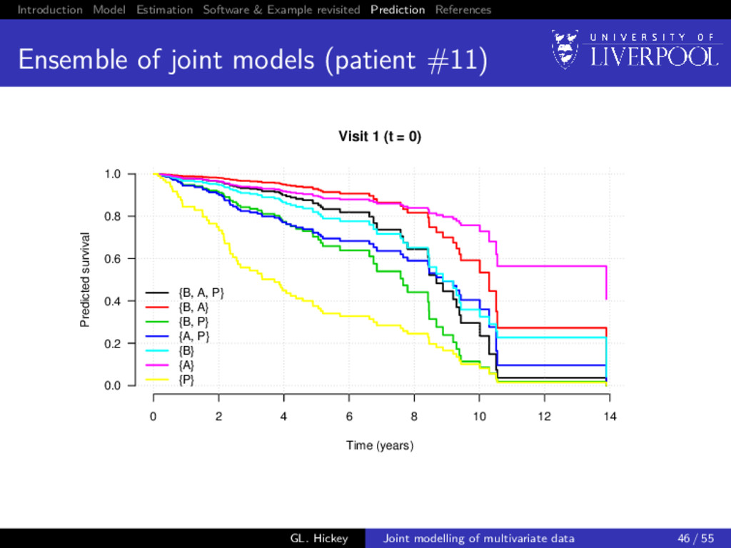
of multiple biomarkers Build all 32 − 1 = 7 joint models: i.e. from trivariate ({B, A, P}) to univariate ({B}, {A}, {P}) For all patients still in the risk set at landmark time (t), predict their failure probability at horizon time (s), i.e. P[t < T∗ i ≤ s + t | T∗ i > t, yi {t}; θ] Calculate concordance statistic7 (Therneau and Watson 2015) between prediction and whether subject had event in (t, s + t] 7Using the survConcordance() function in the R survival package GL. Hickey Joint modelling of multivariate data 45 / 55
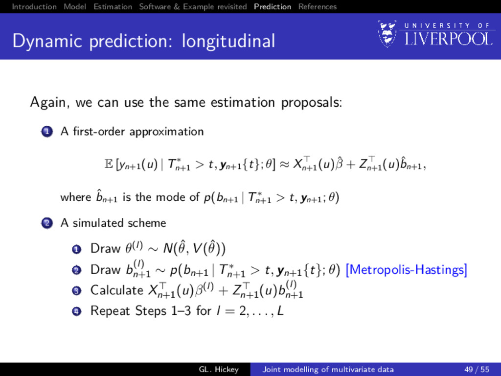
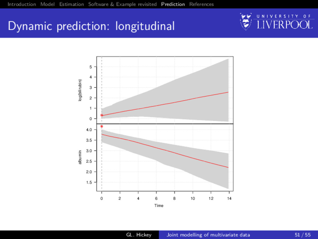
prediction: longitudinal For a new subject i = n + 1, we want to calculate E yn+1(u) | T∗ n+1 > t, yn+1{t}; θ = Xn+1 (u)β + Zn+1 (u)E[bn+1], GL. Hickey Joint modelling of multivariate data 48 / 55
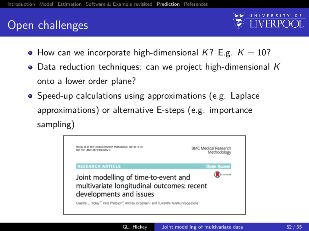
challenges How can we incorporate high-dimensional K? E.g. K = 10? Data reduction techniques: can we project high-dimensional K onto a lower order plane? Speed-up calculations using approximations (e.g. Laplace approximations) or alternative E-steps (e.g. importance sampling) GL. Hickey Joint modelling of multivariate data 52 / 55
I Murtaugh, Paul A et al. (1994). Primary biliary cirrhosis: prediction of short-term survival based on repeated patient visits. Hepatology 20(1), pp. 126–134. Henderson, R et al. (2000). Joint modelling of longitudinal measurements and event time data. Biostatistics 1(4), pp. 465–480. Laird, NM and Ware, JH (1982). Random-effects models for longitudinal data. Biometrics 38(4), pp. 963–74. Andrinopoulou, Eleni-Rosalina and Rizopoulos, Dimitris (2016). Bayesian shrinkage approach for a joint model of longitudinal and survival outcomes assuming different association structures. Statistics in Medicine 35(26), pp. 4813–4823. Andrinopoulou, Eleni-Rosalina, Eilers, Paul H C, et al. (2017). Improved dynamic predictions from joint models of longitudinal and survival data with time-varying effects using P-splines. Biometrics. Dempster, AP et al. (1977). Maximum likelihood from incomplete data via the EM algorithm. J Roy Stat Soc B 39(1), pp. 1–38. Wei, GC and Tanner, MA (1990). A Monte Carlo implementation of the EM algorithm and the poor man’s data augmentation algorithms. J Am Stat Assoc 85(411), pp. 699–704. Ripatti, S et al. (2002). Maximum likelihood inference for multivariate frailty models using an automated Monte Carlo EM algorithm. Life Dat Anal 8(2002), pp. 349–360. GL. Hickey Joint modelling of multivariate data 54 / 55
II Hsieh, F et al. (2006). Joint modeling of survival and longitudinal data: Likelihood approach revisited. Biometrics 62(4), pp. 1037–1043. McLachlan, GJ and Krishnan, T (2008). The EM Algorithm and Extensions. Second. Wiley-Interscience. Rizopoulos, Dimitris (2011). Dynamic predictions and prospective accuracy in joint models for longitudinal and time-to-event data. Biometrics 67(3), pp. 819–829. Therneau, Terry M and Watson, David A (2015). The concordance statistic and the Cox model. Tech. rep. Rochester, Minnesota: Department of Health Science Research, Mayo Clinic, Technical Report Series No. 85. GL. Hickey Joint modelling of multivariate data 55 / 55