Checking model assumptions with regression diagnostics

Checking model
assumptions
with regression
diagnostics
Graeme L. Hickey
University of Liverpool
@graemeleehickey
www.glhickey.com
[email protected]

View Slide

Conflicts of interest
• None
• Assistant Editor (Statistical Consultant) for EJCTS and ICVTS

View Slide

View Slide

Question: who routinely checks model assumptions
when analyzing data?
(raise your hand if the answer is Yes)

View Slide

Outline
• Illustrate with multiple linear regression
• Plethora of residuals and diagnostics for other model types
• Focus is not to “what to do if you detect a problem”, but “how to
diagnose (potential) problems”

View Slide

My personal experience*
• Reviewer of EJCTS and ICVTS for 5-years
• Authors almost never report if they assessed model assumptions
• Example: only one paper submitted where authors considered
sphericity in RM-ANOVA at first submission
• Usually one or more comment is sent to authors regarding model
assumptions
* My views do not reflect those of the EJCTS, ICVTS, or of other statistical reviewers

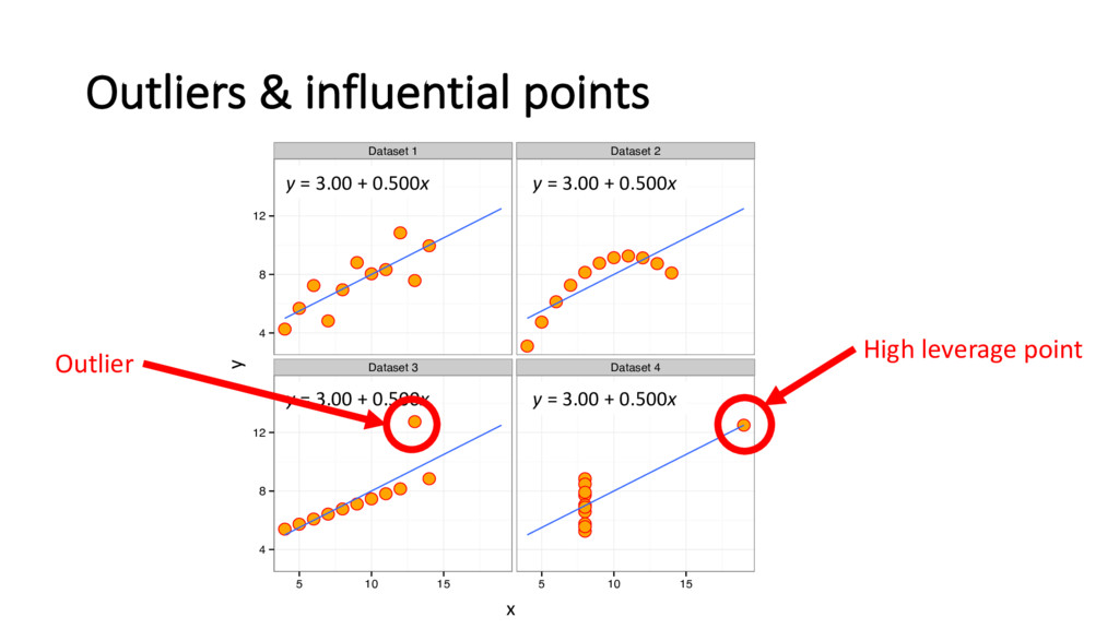
View Slide

Linear regression modelling
• Collect some data
• ": the observed continuous outcome for subject (e.g. biomarker)
• %"
, '"
, … , )": p covariates (e.g. age, male, …)
• Want to fit the model
• "
= ,
+ %
%"
+ '
"'
+ ⋯ + )
)"
+ "
• Estimate the regression coefficients
•
0
,
,
0
%
,
0
'
, … ,
0
)
• Report the coefficients and make inference, e.g. report 95% CIs
• But we do not stop there…

View Slide

Residuals
• For a linear regression model, the residual for the -th observation is
"
= "
−
3"
• where
3" is the predicted value given by

3"
=
0
,
+
0
%
%"
+
0
'
"'
+ ⋯ +
0
)
)"
• Lots of useful diagnostics are based on residuals

View Slide

Linearity of functional form
• Assumption: scatterplot of ("
, "
) should not show any systematic
trends
• Trends imply that higher-order terms are required, e.g. quadratic,
cubic, etc.

View Slide

●●
●
●
●
●
●
●
●
●
●
●
●
●
●
●
●
●
●
●
●
●
●
●
●
●
●
●
●
●
●
●
●
●
●
●
●
●
●
●
●
●
●
●
●
●
●
●
●
●
●
●
● ●
●
●
●
●
●
●
●
●
●
●
●
●
●
●
●
●
●
●
●
●
●
●
●
●
●
●
●
●
●
●
●
●
●
●
●
●
●●
●
●
●
●
●
●
●
●
0
20
40
60
80
0 5 10 15 20
X
Y
A
●
●
●
●
●
●
●
●
●
●
●
●
● ●
●
●
● ●
●
●
●
●
●
●
●
●
●
●
●
●
●
●
●
●
●
●
●
●
●
● ●
●
●
●
●
●
●
●
●
●
●
●
●
●
●
●
●
●
●
●
●
●
●
●
●
●
●
●
●
●
●
●
●
●
●
●
●
●
●
●
●
●
●
●
●
●
●
●
● ●
●
●
●
●
●
●
●
●
●
●
−10
−5
0
5
10
0 5 10 15 20
X
Residual
B
●●
●
●
●
●
●
●
●
●
●
●
●
●
●
●
●
●
●
●
●
●
●
●
●
●
●
●
●
●
●
●
●
●
●
●
●
●
●
●
●
●
●
●
●
●
●
●
●
●
●
●
● ●
●
●
●
●
●
●
●
●
●
●
●
●
●
●
●
●
●
●
●
●
●
●
●
●
●
●
●
●
●
●
●
●
●
●
●
●
●
●
●
●
●
●
●
●
●
●
0
20
40
60
80
0 5 10 15 20
X
Y
C
●
●
●
●
●
●
●
●
●
●
●
●
● ●
●
●
●
●
●
●
●
●
●
●
●
●
●
●
●
●
●
●
●
●
●
●
●
●
●
●
●
●
●
●
●
●
●
●
●
●
●
●
●
●
●
●
●
●
●
●
●
●
●
●
●
●
●
●
●
● ●
●
●
●
●
●
●
●
●
●
●
●
●
●
●
●
●
●
●
●
●
●
●
●
●
●
●
●
●
●
−4
0
4
8
0 5 10 15 20
X
Residual
D
Fitted model:
= ,
+ %
+
= ,
+ %
+ '
' +

View Slide

Homogeneity
• We often assume assume that "
∼ 0, '
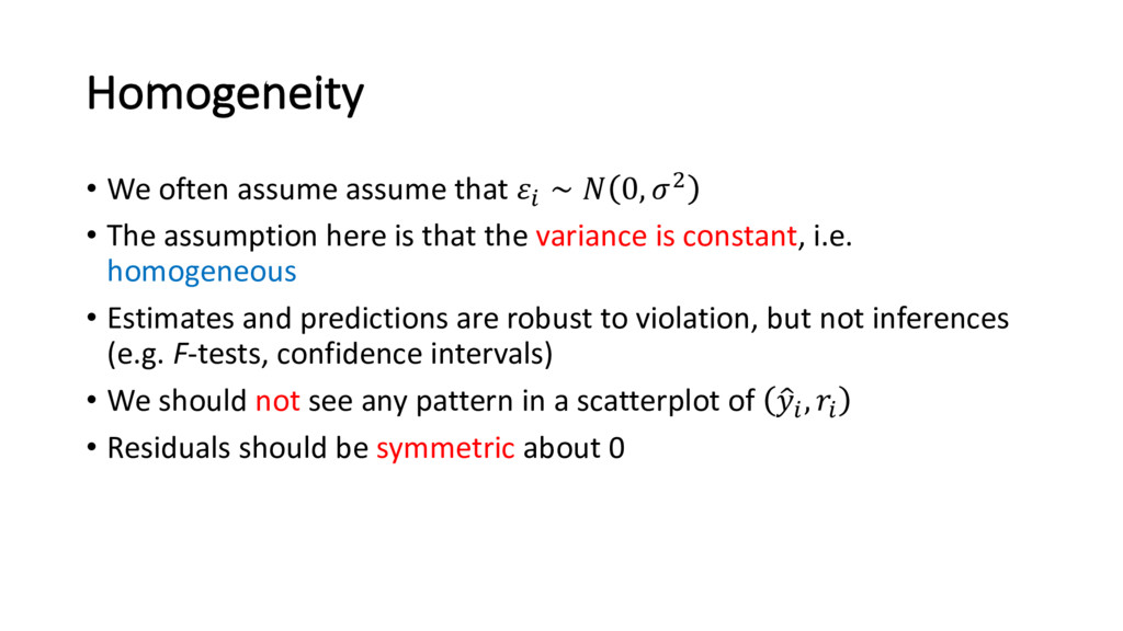
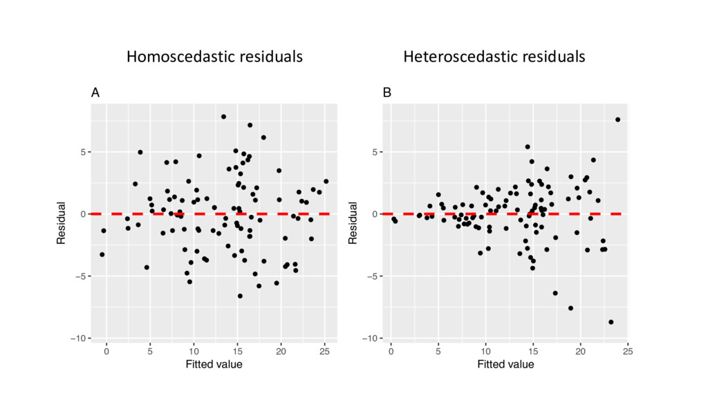
• The assumption here is that the variance is constant, i.e.
homogeneous
• Estimates and predictions are robust to violation, but not inferences
(e.g. F-tests, confidence intervals)
• We should not see any pattern in a scatterplot of
3"
, "
• Residuals should be symmetric about 0

View Slide

Homoscedastic residuals Heteroscedastic residuals
●
●
●
●
●
● ●
●
●
●
●
●
● ●
●
●
●
●
●
●
●
●
●
●
●
●
●
●
●
●
●
●
●
●
●
●
●
●
●
●
●
●
●
●
●
●
●
●
●
●
●
●
●
●
●
●
●
●
●
● ●
●
●
●
●
●
●
●
●
●
●
●
●
●
●
●
●
●
●
●
●
●
●
●
●
●
●
●
●
●
●
●
●
●
●
●
●
●
●
●
−10
−5
0
5
0 5 10 15 20 25
Fitted value
Residual
A
●
●
●
●
●
●
●
●
●
●
●
●
●
●
●
●
●
●
●
●
●
●
●
●
●
●
●
●
●
● ●
●
●
●
●
●
●
●
●
●
●
● ●
●
●
●
●
●
●
●
●
●
●
●
●
●
● ●
●
●
●
●
●
●
●
●
●
●
●
●
●
●
●
●
●
●
●
●
●
●
●
●
●
●
●
●
●
●
●
●
●
●
●
●
●
●
●
●
●
●
−10
−5
0
5
0 5 10 15 20 25
Fitted value
Residual
B

View Slide

Normality
• If we want to make inferences, we generally assume "
∼ 0, '
• Not always a critical assumption, e.g.:
• Want to estimate the ‘best fit’ line
• Want to make predictions
• The sample size is quite large and the other assumptions are met
• We can assess graphically using a Q-Q plot, histogram
• Note: the assumption is about the errors, not the outcomes "

View Slide

●
●
●
●
●
●
●
●
●
●
●
●
●
●
●
●
●
●
●
●
●
●
●
●
●
●
●
●
●
●
●
●
●
●
●
●
●
●
●
●
●
●
●
●
●
●
●
●
●
●
●
●
●
●
●
●
●
●
●
●
●
●
●
●
●
●
●
●
●
●
●
●
●
●
●
●
●
●
●
●
●
●
●
●
●
●
●
●
●
●
●
●
●
●
●
●
●
●
●
●
−2 −1 0 1 2
−6 −2 2 4 6
Normal residuals
Theoretical Quantiles
Sample Quantiles
●
●
●
●
●
●
●
●
● ●
●
●
●
●
● ●
●
●
●
●
● ●
●●
●
●
●
●
●
●
● ●
●
●
●
●
●
●
●
● ●
●
●
●●
●
●
●
●
●
● ●
●
●
●
●
●
●
●
●
●
●
●
●
● ●
●
●
●
●
●
●
●
●
●
●
●
●
●
●
●
●
●
●
●
●
●
●
●
●
●
●
●
●
●
●
●
●
●
●
−2 −1 0 1 2
0 5 10 15
Skewed residuals
Theoretical Quantiles
Sample Quantiles
Residuals
Frequency
−6 −4 −2 0 2 4 6 8
0 5 10 15 20 25
Residuals
Frequency
0 5 10 15
0 5 10 20 30

View Slide

Independence
• We assume the errors are independent
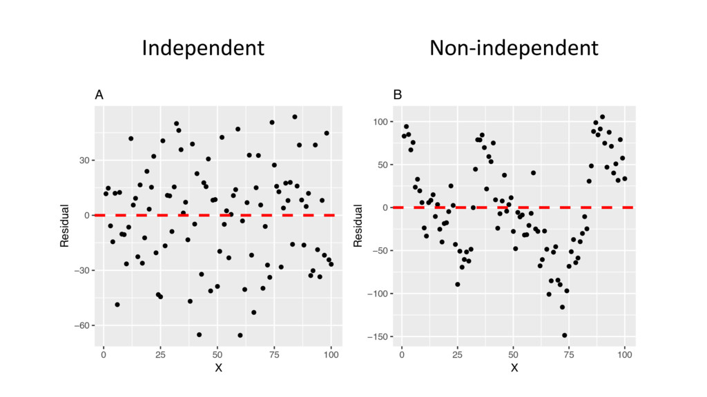
• Usually able to identify this assumption from the study design and
analysis plan
• E.g. if repeated measures, we should not treat each measurement as
independent
• If independence holds, plotting the residuals against the time (or
order of the observations) should show no pattern

View Slide

●
●
●
●
●
●
●
●
●
●
●
●
●
●
●
●
●
●
●
●
●
●
●
●
●
●
●
●
●
●
●
●
●
●
●
●
●
●
●
●
●
●
●
●
●
●
●
●
●
●
●
●
●
●
●
●
●
●
●
●
●
●
●
●
●
●
●
●
●
●
●
●
●
●
●
●
●
●
●
●
●
●
●
●
●
●
●
●
●
●
●
●
●
●
●
●
●
●
●
●
−60
−30
0
30
0 25 50 75 100
X
Residual
A
●
●
●
●
●
●
●
●
●
●
●
●
●
●
●
●
●
●
●
●
●
●
●
●
●
●
●
●
●
●
●
●
●
●
●
●
●
●
●
●
●
●
●
●
●
●
●
●
●
●
●
●
●
●
●
●
●
●
●
●
●
●
●
●
●
●
●
●
●
●
●
●
●
●
●
●
●
●
●
●
●
●
●
●
●
●
●
●
●
●
●
●
●
●
●
●
●
●
●
●
−150
−100
−50
0
50
100
0 25 50 75 100
X
Residual
B
Independent Non-independent

View Slide

Multicollinearity
• Correlation among the predictors (independent variables) is known as
collinearity (multicollinearity when >2 predictors)
• If aim is inference, can lead to
• Inflated standard errors (in some cases very large)
• Nonsensical parameter estimates (e.g. wrong signs or extremely large)
• If aim is prediction, it tends not to be a problem
• Standard diagnostic is the variance inflation factor (VIF)
?
=
1
1 − ?
' Rule of thumb: VIF > 10 indicates multicollinearity

View Slide

Outliers & influential points
●
●
●
● ●
●
●
●
●
●
●
r = 0.82
●
●
●
● ●
●
●
●
●
●
●
r = 0.82
●
●
●
●
●
●
●
●
●
●
●
r = 0.82
●
●
●
●
●
●
●
●
●
●
●
r = 0.82
Dataset 1 Dataset 2
Dataset 3 Dataset 4
4
8
12
4
8
12
5 10 15 5 10 15
Measurement 1
Measurement 2
y = 3.00 + 0.500x y = 3.00 + 0.500x
y = 3.00 + 0.500x y = 3.00 + 0.500x
x
y
Outlier
High leverage point

View Slide

Diagnostics to detect influential points
• DFBETA (or Δβ)
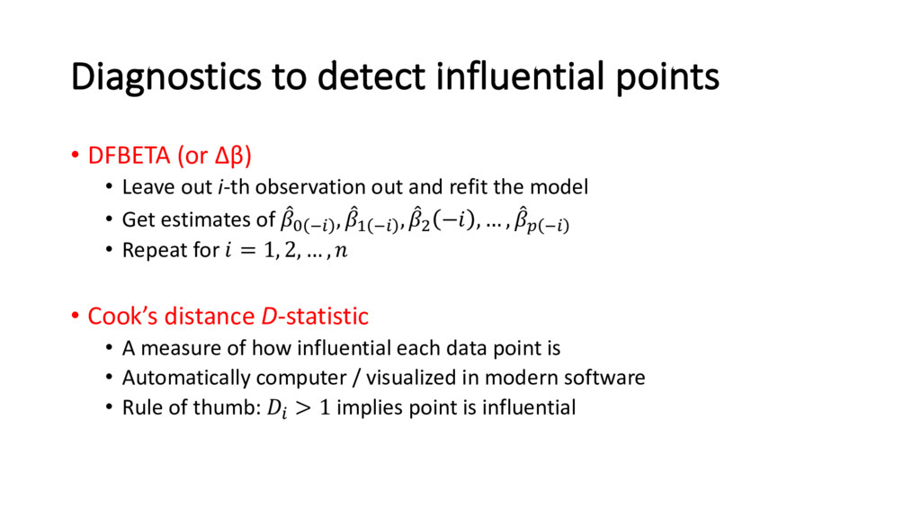
• Leave out i-th observation out and refit the model
• Get estimates of
0
, C"
,
0
% C"
,
0
'
− , … ,
0
) C"
• Repeat for = 1, 2, … ,
• Cook’s distance D-statistic
• A measure of how influential each data point is
• Automatically computer / visualized in modern software
• Rule of thumb: "
> 1 implies point is influential

View Slide

Residuals from other models
GLMs (incl. logistic regression)
• Deviance
• Pearson
• Response
• Partial
• Δβ
• …
Cox regression
• Martingale
• Deviance
• Score
• Schoenfeld
• Δβ
• …
Useful for exploring the influence of individual observations and model fit

View Slide

Two scenarios
Statistical methods routinely submitted to EJCTS / ICVTS include:
1. Repeated measures ANOVA
2. Cox proportional hazards regression
Each has very important assumptions

View Slide

Repeated measures ANOVA
• Assumptions: those used for classical ANOVA + sphericity
• Sphericity: the variances of the differences of all pairs of the within
subject conditions (e.g. time) are equal
• It’s a questionable a priori assumption for longitudinal data
Patient T0 T1 T2 T0 – T1 T0 – T2 T1 – T2
1 30 27 20 3 10 7
2 35 30 28 5 7 2
3 25 30 20 −5 5 10
4 15 15 12 0 3 3
5 9 12 7 −3 2 5
Variance 17.0 10.3 10.3

View Slide

Mauchly's test
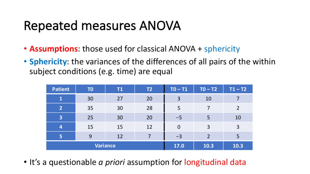
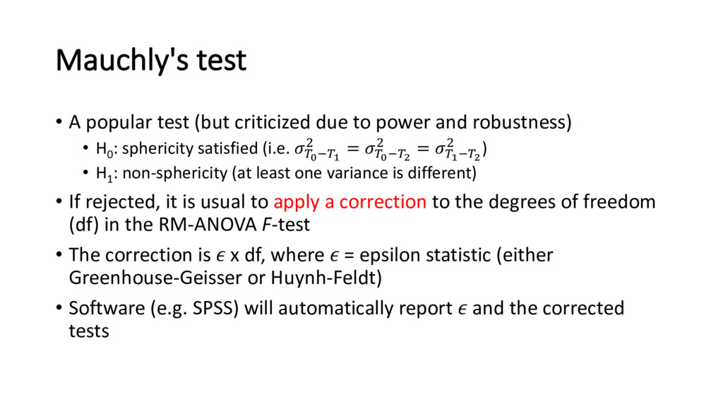
• A popular test (but criticized due to power and robustness)
• H0
: sphericity satisfied (i.e. HICHJ
' = HICHK
' = HJCHK
' )
• H1
: non-sphericity (at least one variance is different)
• If rejected, it is usual to apply a correction to the degrees of freedom
(df) in the RM-ANOVA F-test
• The correction is x df, where = epsilon statistic (either
Greenhouse-Geisser or Huynh-Feldt)
• Software (e.g. SPSS) will automatically report and the corrected
tests

View Slide

Proportionality assumption
• Cox regression assumes proportional hazards:
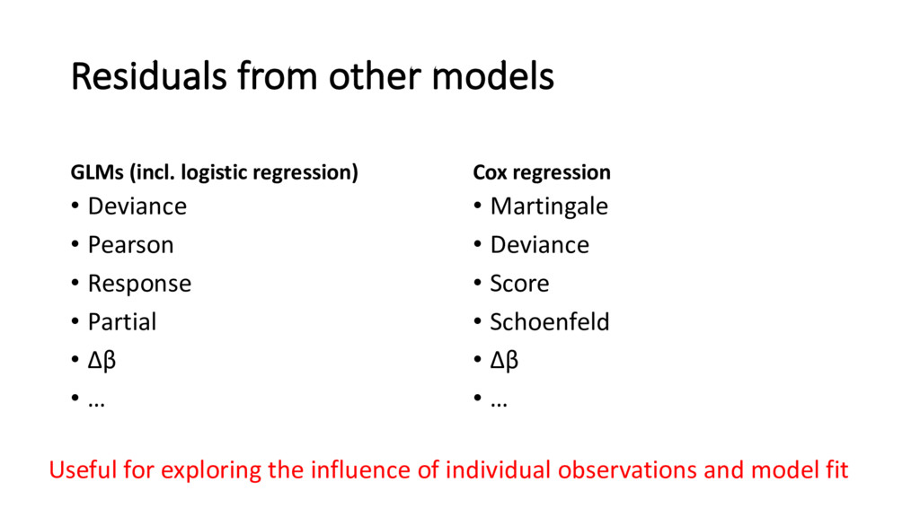
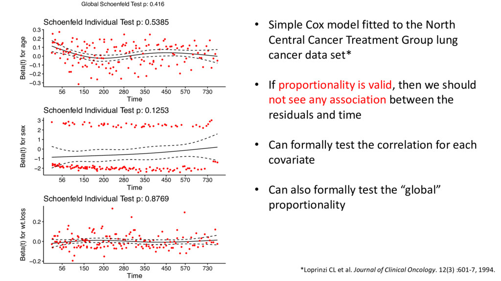
• Equivalently, the hazard ratio must be constant over time
• There are many ways to assess this assumption, including two using
residual diagnostics:
• Graphical inspection of the (scaled) Schoenfeld residuals
• A test* based on the Schoenfeld residuals
* Grambsch & Therneau. Biometrika. 1994; 81: 515-26.

View Slide

●
●
●
●
●
●
●
●
●
●
●
●
●
●
●
●
●
●
●
●
●
●
●
●
●
●
●
●
●
●
●
●
●
●
●
●
●
●
●
●
●
●
●
●
●
●
●
●
●
●
●
●
●
●
●
●
●
●
●
●
●
●
●
●
●
●
●
●
●
●
●
●
●
●
●
●
●
●
●
●
●
●
●
●
●
●
●
●
●
●
●
●
●
●
●
●
●
●
●
●
●
●
●
●
●
●
●
●
●
●
●
●
●●
●
●
●
●
●
●
●
●
●●
●
●
●
●
●
●
●●
●
●
●
●
●
●
●
●
●
●●
●
●
●
●
●
●
●
●
●
−0.3
−0.2
−0.1
0.0
0.1
0.2
0.3
56 150 200 280 350 450 570 730
Time
Beta(t) for age
Schoenfeld Individual Test p: 0.5385
●
●
●●
●
●●
●
●
●
●
●●
●
●
●
●
●
●
●
●
●
●
●
●
●
●
●
●●
●
●
●
●
●
●
●
●
●
●
●
●
●
●
●
●
●
●
●
●
●
●
●
●
●
●
●
●
●
●
●
●
●
●
●
●
●
●
●
●
●
●
●
●
●
●
●
●
●
●
●
●
●
●
●
●
●
●
●
●
●
●
●
●
●
●
●
●
●
●●●
●
●
●
●
●
●
●●
●
●
●
●
●
●
●
●
●●
●
●
●
●
●
●
●
●
●
●
●
●●
●
●●
●
●
●
●
●
●
●
●
●
●
●
●
●
● ● ●
−2
−1
0
1
2
3
56 150 200 280 350 450 570 730
Time
Beta(t) for sex
●
●
●
●
●
●●
●
●
●
●
●
●
●
●
●
●
●
●
●
●
●
●
●
●
●
●
●
●
●
●
●
●
●
●
●
●
●
●
●
●
●
●
●
●
●
●
●
●
●
●
●
●●
●
●
●
●
●
●
●
●
●
●
●
●
●
●
●
●
●
●
●
●
●
●
●
●
●
●
●
●
●
●
●
●
●
●
●
●
●
●
●
●
●
●
●
●
●
●
●
●●
●
● ●
●
●
●
●
●
●
●
●
●
●
●
●
●
●
●
●
●
●●
●
●
●
●
●
●
●
●
●
●
●
●
●●
●
●
●
●
●
●
●
●
●
● ●
●
●
−0.2
0.0
0.2
56 150 200 280 350 450 570 730
Time
Beta(t) for wt.loss
Global Schoenfeld Test p: 0.416
• Simple Cox model fitted to the North
Central Cancer Treatment Group lung
cancer data set*
• If proportionality is valid, then we should
not see any association between the
residuals and time
• Can formally test the correlation for each
covariate
• Can also formally test the “global”
proportionality
*Loprinzi CL et al. Journal of Clinical Oncology. 12(3) :601-7, 1994.

View Slide

Conclusions
• Residuals are incredibly powerful for diagnosing issues in regression
models
• If a model doesn’t satisfy the required assumptions, don’t expect
subsequent inferences to be correct
• Assumptions can usually be assessed using methods other than (or in
combination with) residuals
• Always report in manuscript
• What diagnostics were used, even if they are absent from the Results section
• Any corrections or adjustments made as a result of diagnostics

View Slide

Slides available (shortly)
from: www.glhickey.com
Thanks for listening
Any questions?
Statistical Primer article
to be published soon!

View Slide

Checking model assumptions with regression diagnostics

Checking model assumptions with regression diagnostics

Graeme Hickey

More Decks by Graeme Hickey

Other Decks in Research

Featured

Transcript