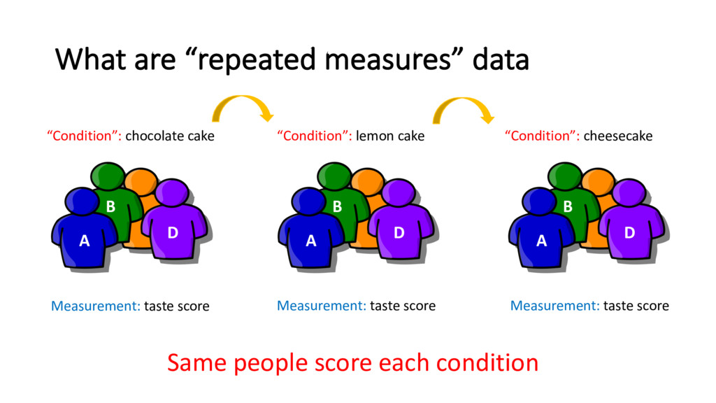
D A B D “Condition”: chocolate cake “Condition”: lemon cake “Condition”: cheesecake Measurement: taste score Measurement: taste score Measurement: taste score Same people score each condition
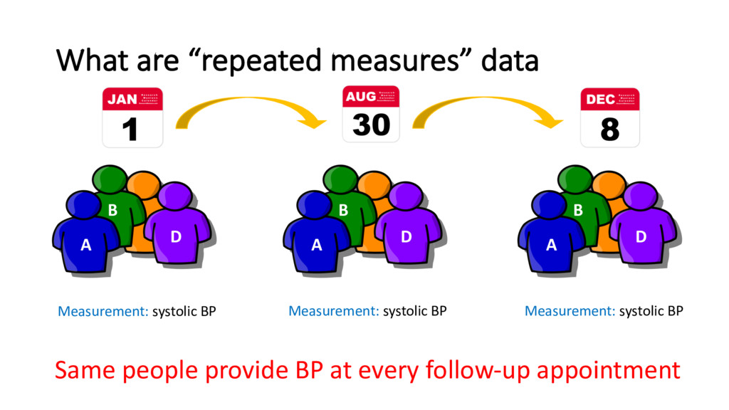
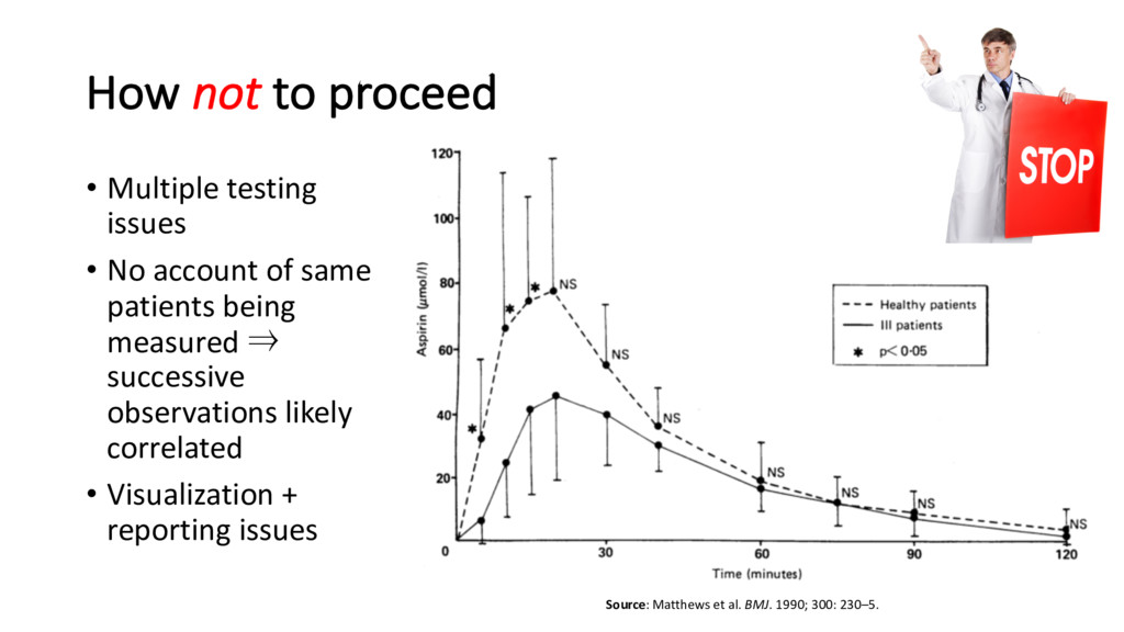
independent: repeated observations on the same individual will be more similar to each other than to observations on other individuals • Guidelines for reporting mortality and morbidity after cardiac valve interventions also propose the use of longitudinal data analysis for repeated measurement data
taken Measurement taken before treatment after treatment A B D E F H E F H Placebo Active treatment Question: if patients are randomised to treatment arms, how can we test whether active treatment is more effective than placebo?
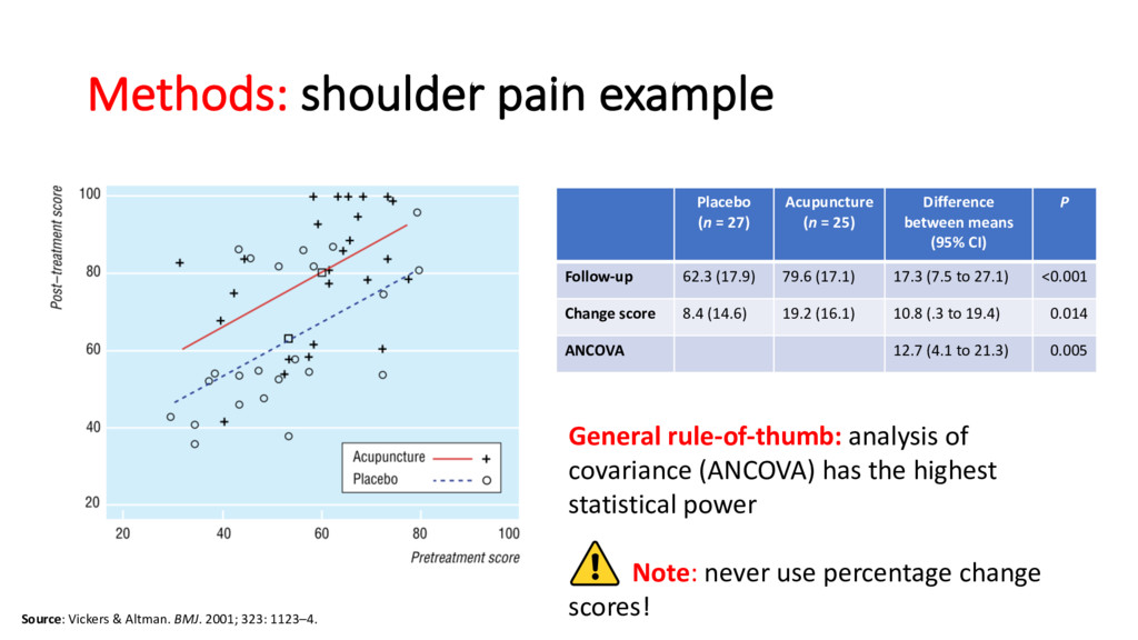
323: 1123–4. Placebo (n = 27) Acupuncture (n = 25) Difference between means (95% CI) P Follow-up 62.3 (17.9) 79.6 (17.1) 17.3 (7.5 to 27.1) <0.001 Change score 8.4 (14.6) 19.2 (16.1) 10.8 (.3 to 19.4) 0.014 ANCOVA 12.7 (4.1 to 21.3) 0.005 General rule-of-thumb: analysis of covariance (ANCOVA) has the highest statistical power Note: never use percentage change scores!
baseline, 1-hr, 2-hr, 8-hr, 16-hr, 24-hr) • Unbalanced (e.g. patient A visits their physician on days 1, 4, 6, 9, 12, and patient B visits only on days 5, 9, and 15) • Missing data • E.g. patient fails to attend scheduled follow-up appointment
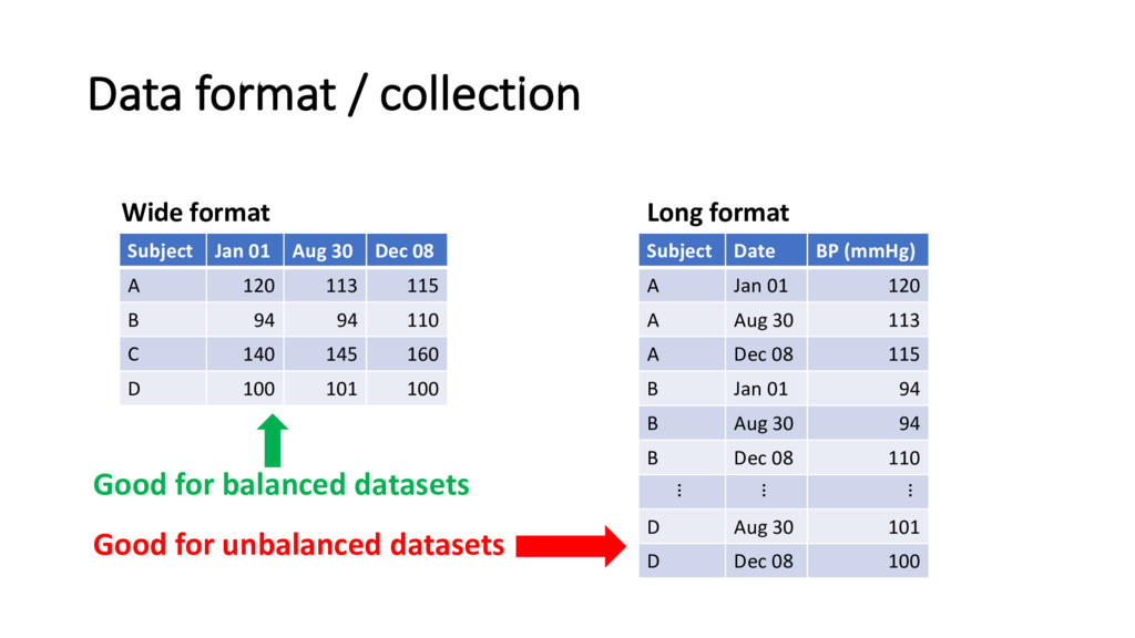
30 Dec 08 A 120 113 115 B 94 94 110 C 140 145 160 D 100 101 100 Long format Subject Date BP (mmHg) A Jan 01 120 A Aug 30 113 A Dec 08 115 B Jan 01 94 B Aug 30 94 B Dec 08 110 ⠇ ⠇ ⠇ D Aug 30 101 D Dec 08 100 Good for balanced datasets Good for unbalanced datasets
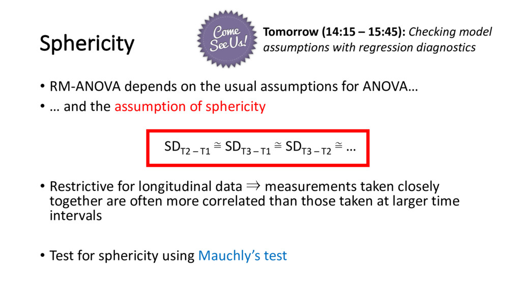
• … and the assumption of sphericity SDT2 – T1 ≅ SDT3 – T1 ≅ SDT3 – T2 ≅ … • Restrictive for longitudinal data ⇒ measurements taken closely together are often more correlated than those taken at larger time intervals • Test for sphericity using Mauchly’s test Tomorrow (14:15 – 15:45): Checking model assumptions with regression diagnostics
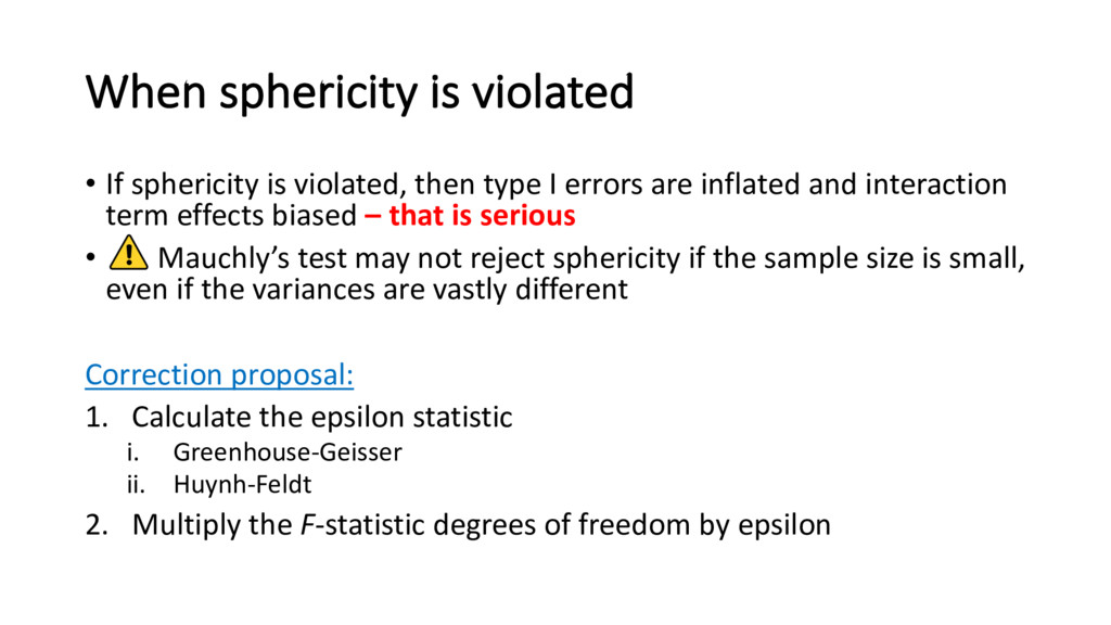
type I errors are inflated and interaction term effects biased – that is serious • Mauchly’s test may not reject sphericity if the sample size is small, even if the variances are vastly different Correction proposal: 1. Calculate the epsilon statistic i. Greenhouse-Geisser ii. Huynh-Feldt 2. Multiply the F-statistic degrees of freedom by epsilon
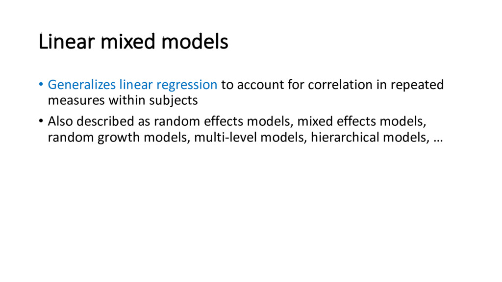
correlation in repeated measures within subjects • Also described as random effects models, mixed effects models, random growth models, multi-level models, hierarchical models, …
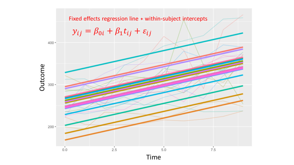
= & + &" + ( + (" "# + "# • &" , (" are called subject-specific random intercepts: intercept and slope respectively, distributed N2 (0, Σ) • Observations within-subjects are more correlated than observations between-subjects • Can be adjusted for other (possibly time-varying) covariates and baseline measurements
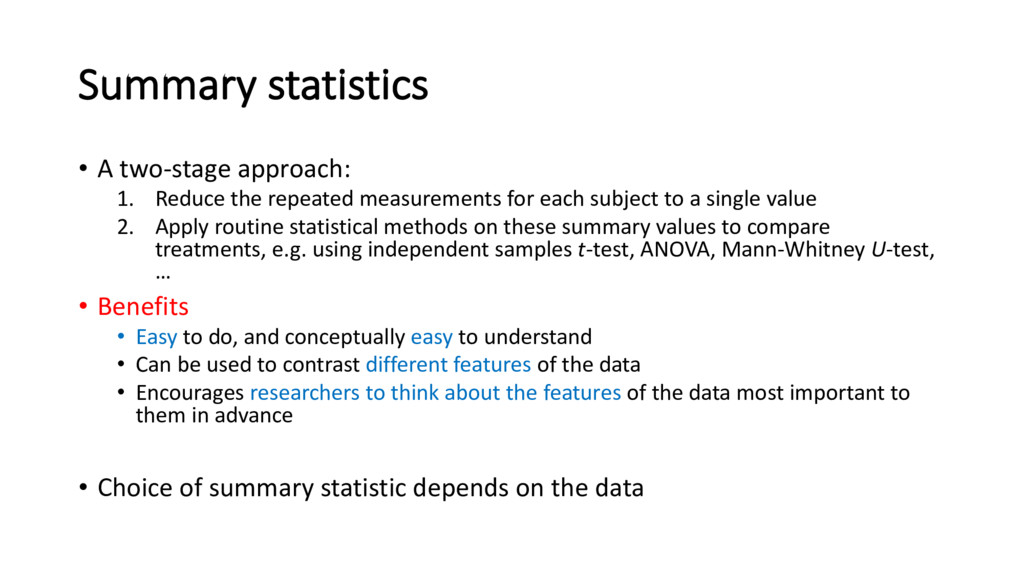
measurements for each subject to a single value 2. Apply routine statistical methods on these summary values to compare treatments, e.g. using independent samples t-test, ANOVA, Mann-Whitney U-test, … • Benefits • Easy to do, and conceptually easy to understand • Can be used to contrast different features of the data • Encourages researchers to think about the features of the data most important to them in advance • Choice of summary statistic depends on the data
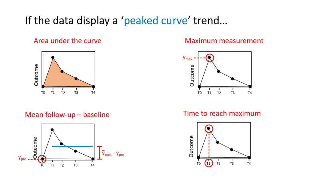
T4 Outcome T2 T0 T1 T3 T4 Outcome ypre T2 ypost - ypre T0 T1 T3 T4 T2 Outcome If the data display a ‘peaked curve’ trend… Area under the curve Maximum measurement Time to reach maximum Mean follow-up – baseline
Final value Time to a certain % increase/decrease Slope T0 T1 T3 T4 Outcome T2 ychange T0 T1 T3 T4 Outcome T2 yfinal T0 T1 T3 T4 Outcome T2 slope T0 T1 T3 T4 T2 Outcome
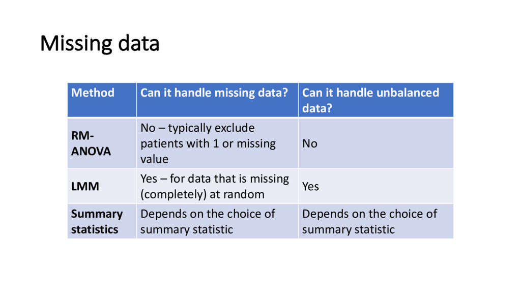
handle unbalanced data? RM- ANOVA No – typically exclude patients with 1 or missing value No LMM Yes – for data that is missing (completely) at random Yes Summary statistics Depends on the choice of summary statistic Depends on the choice of summary statistic
![Performing repeated measures analysis Graeme L. Hickey @graemeleehickey www.glhickey.com [email protected]](https://files.speakerdeck.com/presentations/9d745f6221904bcf8f38cf0e4fef72bf/slide_0.jpg)