A comparison of joint models for longitudinal and competing risks data, with application to an epilepsy drug randomized controlled trial

Department of Biostatistics Seminar, University of Liverpool

Transcript

1. models With application to an epilepsy drug randomized controlled trial
2. http://bit.ly/2FU7wWA
3. S A N A D
4. Secondary objective:
5. • Observed failure time !" • Event indicator #"
7. The response:
8. ! " # $ %" ($) ( " # ($) )" ($) ! "* + $ ,"* ($) ( "* + ($) g = 1,…,G Time-to-event Longitudinal - # -* + ." , 0" 1" ($)
9. • Longitudinal sub-model ! " # $"% &"' + &"# $"% • Time-to-event sub-model
10. 1. The longitudinal sub-model: 2. The time-to-event sub-model:
12. Model Reference 1 Williamson PR et al. Joint modelling of longitudinal and competing risks data. Stat Med. 2008;27: 6426–6438. 2 Elashoff RM et al. A joint model for longitudinal measurements and survival data in the presence of multiple failure types. Biometrics. 2008;64: 762–771. 3 Rizopoulos D. Joint Models for Longitudinal and Time-to-Event Data, with Applications in R. Boca Raton, FL: Chapman & Hall/CRC; 2012. 4 Proust-Lima C et al. Joint modelling of repeated multivariate cognitive measures and competing risks of dementia and death: a latent process and latent class approach. Stat Med. 2015; In press. Only ones with code / software packages available* * at time of writing the manuscript
13. Model Baseline hazards Software Estimation algorithm 1 Non-parametric (unspecified) R code MLE (EM algorithm) + bootstrap for SE / CIs 2 Non-parametric (unspecified) C code MLE (EM algorithm) 3 B-spline basis (on log-hazard scale) R package (JM) MLE (EM + Newton-Raphson algorithm) 4a Weibull R package (lcmm) MLE (Marquardt algorithm) 4b Piecewise constant 4c Cubic M-splines
14. Model Type ! "# $ % 1 Current value of latent process parameterization &# ! " ' (%) 2 Random effects parameterization &# *" with &' = 1, Cov ." , *" = Σ23 and Var * = 73 8 3a Current value parameterization &# 9" % 3b Time-dependent slopes parameterization &# (')9" % + &# (8) ; ;% 9" % 3c Lagged-effects parameterization &# 9" max{% − @, 0} 3d Cumulative effects parameterization &# C D E 9" F ;F 3e Weighted-cumulative effects parameterization &# C D E G(% − F)9" F ;F 3f Special case of the random effects parameterization (with fixed component) &# H ' ' + ."' 4 Association between sub-models accounted entirely for by latent classes N/A
15. Y(t) μ(t) X Z(t)Tb T ε ⍺ g (β2 (1), β3 (1)) βg (2) Y(t) μ(t) X Z(t)Tb T ε ⍺ g (β2 (1), β3 (1)) βg (2) Model 1 Models 3a, c Y(t) μ(t) X Z(t)Tb T ε ⍺ g (1) (β2 (1), β3 (1)) βg (2) Models 3b, d, e ⍺ g (2) Y(t) μ(t) X Z(t)Tb T ε ⍺ g (β2 (1), β3 (1)) βg (2) Model 3f
16. • Basic idea: • R
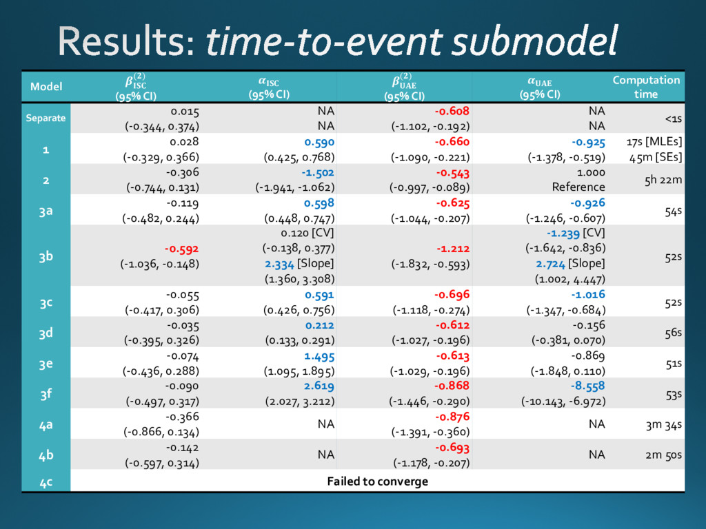
17. Model ! "#$ (&) (95% CI) ("#$ (95% CI) ! )*+ (&) (95% CI) ()*+ (95% CI) Computation time Separate 0.015 (-0.344, 0.374) NA NA -0.608 (-1.102, -0.192) NA NA <1s 1 0.028 (-0.329, 0.366) 0.590 (0.425, 0.768) -0.660 (-1.090, -0.221) -0.925 (-1.378, -0.519) 17s [MLEs] 45m [SEs] 2 -0.306 (-0.744, 0.131) -1.502 (-1.941, -1.062) -0.543 (-0.997, -0.089) 1.000 Reference 5h 22m 3a -0.119 (-0.482, 0.244) 0.598 (0.448, 0.747) -0.625 (-1.044, -0.207) -0.926 (-1.246, -0.607) 54s 3b -0.592 (-1.036, -0.148) 0.120 [CV] (-0.138, 0.377) 2.334 [Slope] (1.360, 3.308) -1.212 (-1.832, -0.593) -1.239 [CV] (-1.642, -0.836) 2.724 [Slope] (1.002, 4.447) 52s 3c -0.055 (-0.417, 0.306) 0.591 (0.426, 0.756) -0.696 (-1.118, -0.274) -1.016 (-1.347, -0.684) 52s 3d -0.035 (-0.395, 0.326) 0.212 (0.133, 0.291) -0.612 (-1.027, -0.196) -0.156 (-0.381, 0.070) 56s 3e -0.074 (-0.436, 0.288) 1.495 (1.095, 1.895) -0.613 (-1.029, -0.196) -0.869 (-1.848, 0.110) 51s 3f -0.090 (-0.497, 0.317) 2.619 (2.027, 3.212) -0.868 (-1.446, -0.290) -8.558 (-10.143, -6.972) 53s 4a -0.366 (-0.866, 0.134) NA -0.876 (-1.391, -0.360) NA 3m 34s 4b -0.142 (-0.597, 0.314) NA -0.693 (-1.178, -0.207) NA 2m 50s 4c Failed to converge
18. 0 1 2 3 4 5 −2 0 2 4 6 8 10 Class−specific mean predicted trajectory Time from randomization (years) Calibrated dose class1 class2 class3 class4 class5 CBZ LTG Longitudinal sub-model Competing risks sub-model Patients distributed 22.8%, 6.6%, 58.3%, 7.4%, and 4.8% for classes 1 to 5, respectively
19. Model Software Speed Other 1 • Currently, only code available – wasn’t in an R package • SEs estimated by bootstrap can be slow • Extends the seminal model by Henderson et al. (2000) 2 • Currently only available as C code files – not standard software choice of biostatisticians • Slow to converge • Constraints on latent association structure complicates interpretation 3 • Available as a comprehensive joint model package in R • Very fast • Flexible range of latent association structures • Fits a contrasts model; i.e. estimates ! and " such that # $ $ = # & $ + ! and ($ = (& + ", respectively 4 • Available as a comprehensive joint model package in R • Need to fit multiple models with different number of classes – moderately slow • Need to fit final model from multiple initial values to ensure reached global maximum – slow • Flexible choice of survival models • Can’t quantify the association between two sub-models • Don’t need to worry about correctly specifying form of ) *+ , -
20. Treatment effects Association parameters
22. Paper, code and data available from www.glhickey.com Project funded by MRC MR/M013227/1 R package joineR now implements Model 1