Lecture slides for POM 1-12

生産管理技術1の講義12のスライドです．

Transcript

1. © Hajime Mizuyama Production & Operations Management #1 @AGU Lec.12: Single and Two-Machine Scheduling • Machine scheduling and Gantt chart • Some single-machine scheduling problems • Johnson’s and Jackson’s algorithm for two-machine case
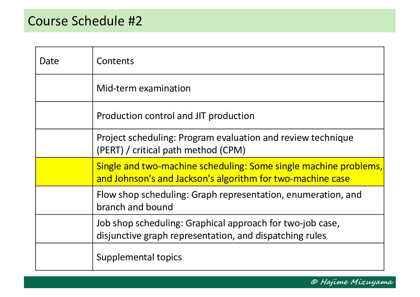
2. © Hajime Mizuyama Course Schedule #2 Date Contents Mid-term examination Production control and JIT production Project scheduling: Program evaluation and review technique (PERT) / critical path method (CPM) Single and two-machine scheduling: Some single machine problems, and Johnson's and Jackson's algorithm for two-machine case Flow shop scheduling: Graph representation, enumeration, and branch and bound Job shop scheduling: Graphical approach for two-job case, disjunctive graph representation, and dispatching rules Supplemental topics
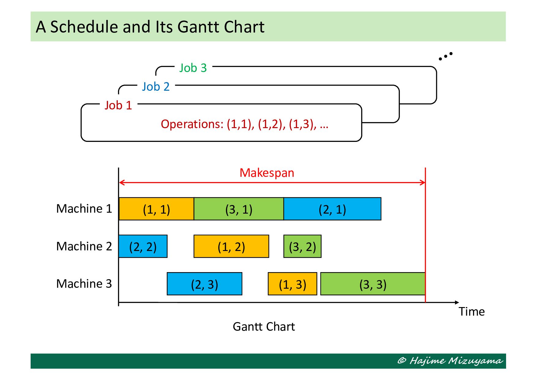
3. © Hajime Mizuyama Machine scheduling is the temporal assignment of jobs to machines to attain some objectives with satisfying specified conditions (constraints). We mainly focus on the makespan as the objective but may deal with some other ones in the following. Terminology • Operation: When a job needs to be processed on two or more machines, the processing of the job on each machine is called an operation. A job may be composed of two or more operations. • Processing route: The prespecified sequence of the machines on which a job is processed; The sequence of the operations of a job. • Makespan: The time length until all the jobs are finished. Machine Scheduling and Some Terminology
4. © Hajime Mizuyama We assume the following unless specified otherwise: • All the jobs are available from the beginning; Their release dates are 0. • Unlimited buffer space is available before and after every machine, and material handling between machines does not take much time. • Pre-emption is not allowed for any job on any machine; Once a machine starts processing a job (or operation), the machine cannot work on another job (or operation) until completing the current one. • Recirculation is not necessary for any job; Each job needs to be processed on each machine at most once. • The setup time necessary for a machine to start a job does not depend on the sequence of jobs on the machine and is included in the processing time of the job on the machine. Some General Assumptions
5. © Hajime Mizuyama A Schedule and Its Gantt Chart Job 3 Job 2 Job 1 Operations: (1,1), (1,2), (1,3), … Machine 1 Machine 2 Machine 3 Time Gantt Chart (1, 1) (1, 2) (1, 3) (2, 2) (2, 1) (2, 3) (3, 3) (3, 2) (3, 1) Makespan
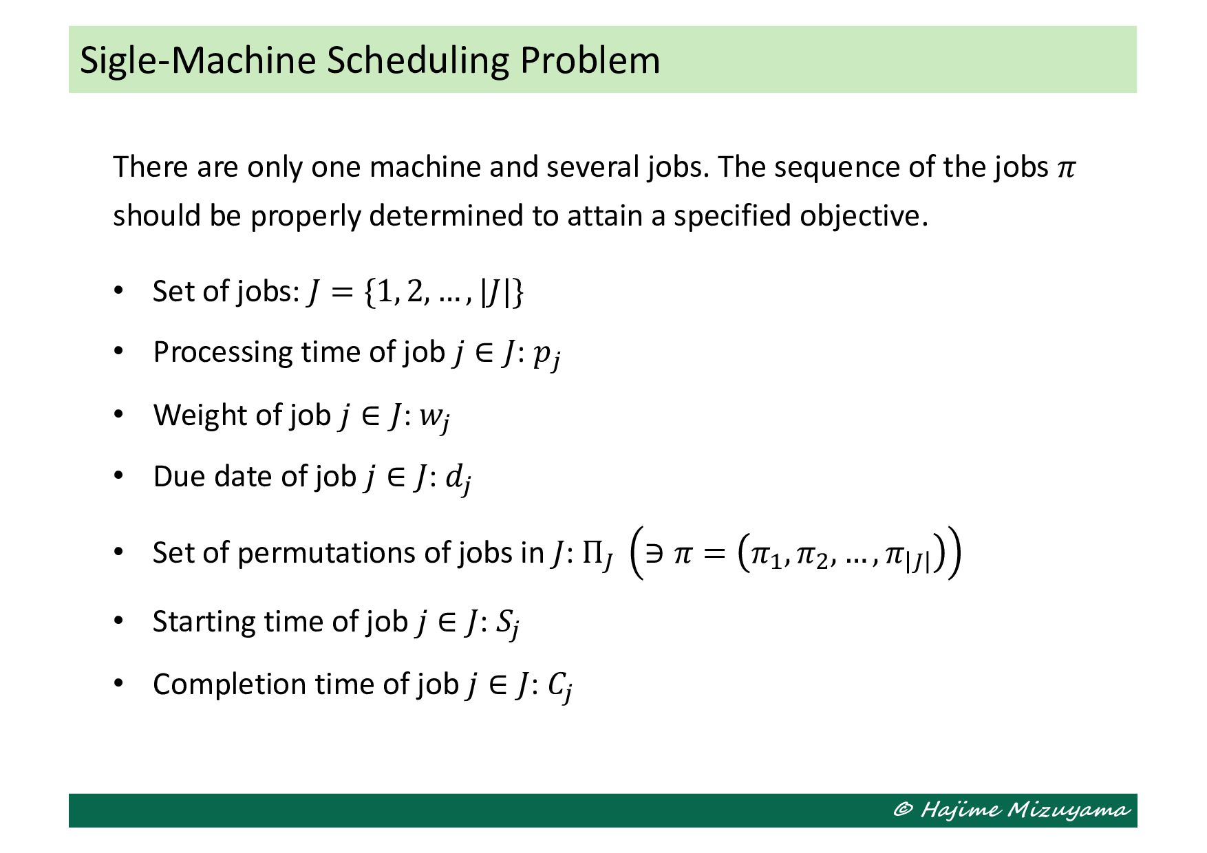
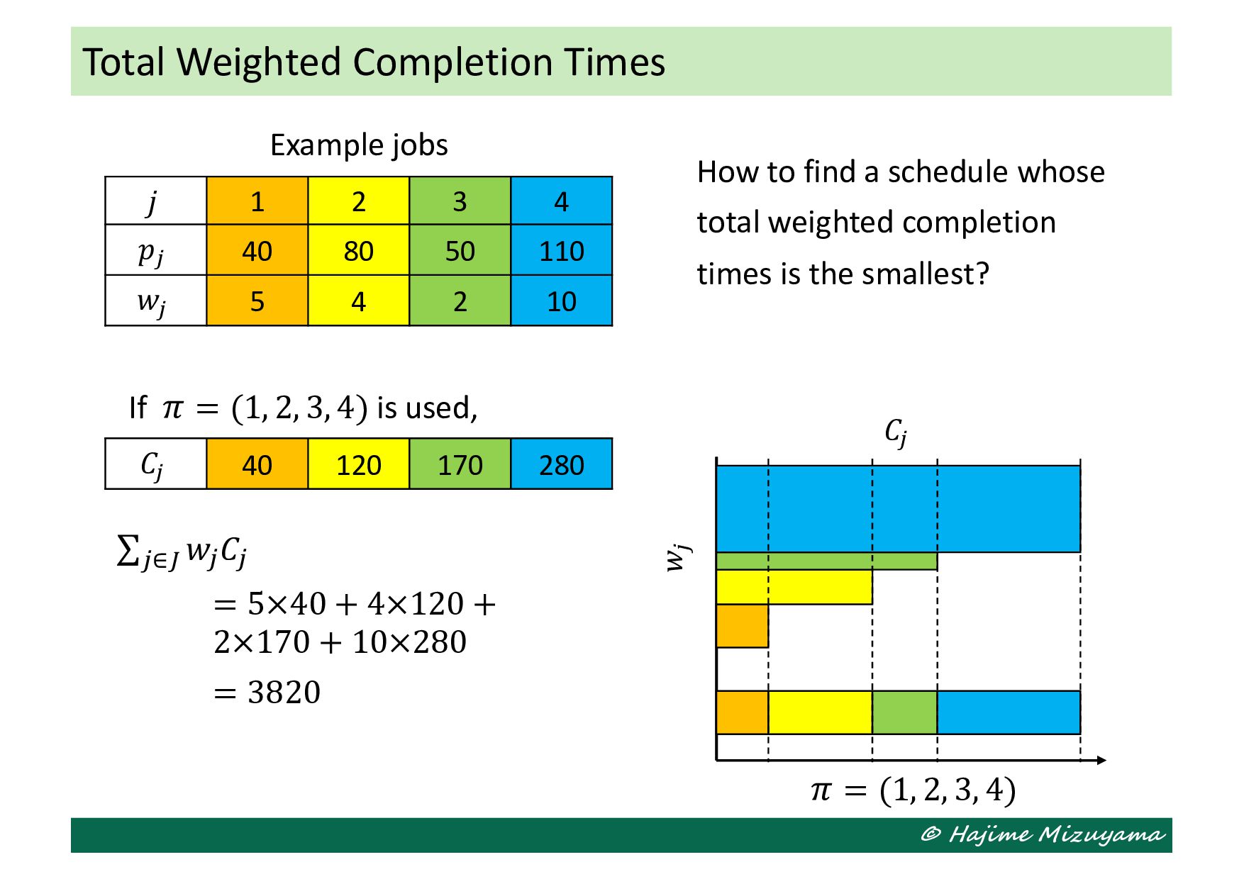
6. © Hajime Mizuyama There are only one machine and several jobs. The sequence of the jobs 𝜋 should be properly determined to attain a specified objective. • Set of jobs: 𝐽 = {1, 2, … , |𝐽|} • Processing time of job 𝑗 ∈ 𝐽: 𝑝! • Weight of job 𝑗 ∈ 𝐽: 𝑤! • Due date of job 𝑗 ∈ 𝐽: 𝑑! • Set of permutations of jobs in 𝐽: Π" ∋ 𝜋 = 𝜋# , 𝜋$ , … , 𝜋 " • Starting time of job 𝑗 ∈ 𝐽: 𝑆! • Completion time of job 𝑗 ∈ 𝐽: 𝐶! Sigle-Machine Scheduling Problem
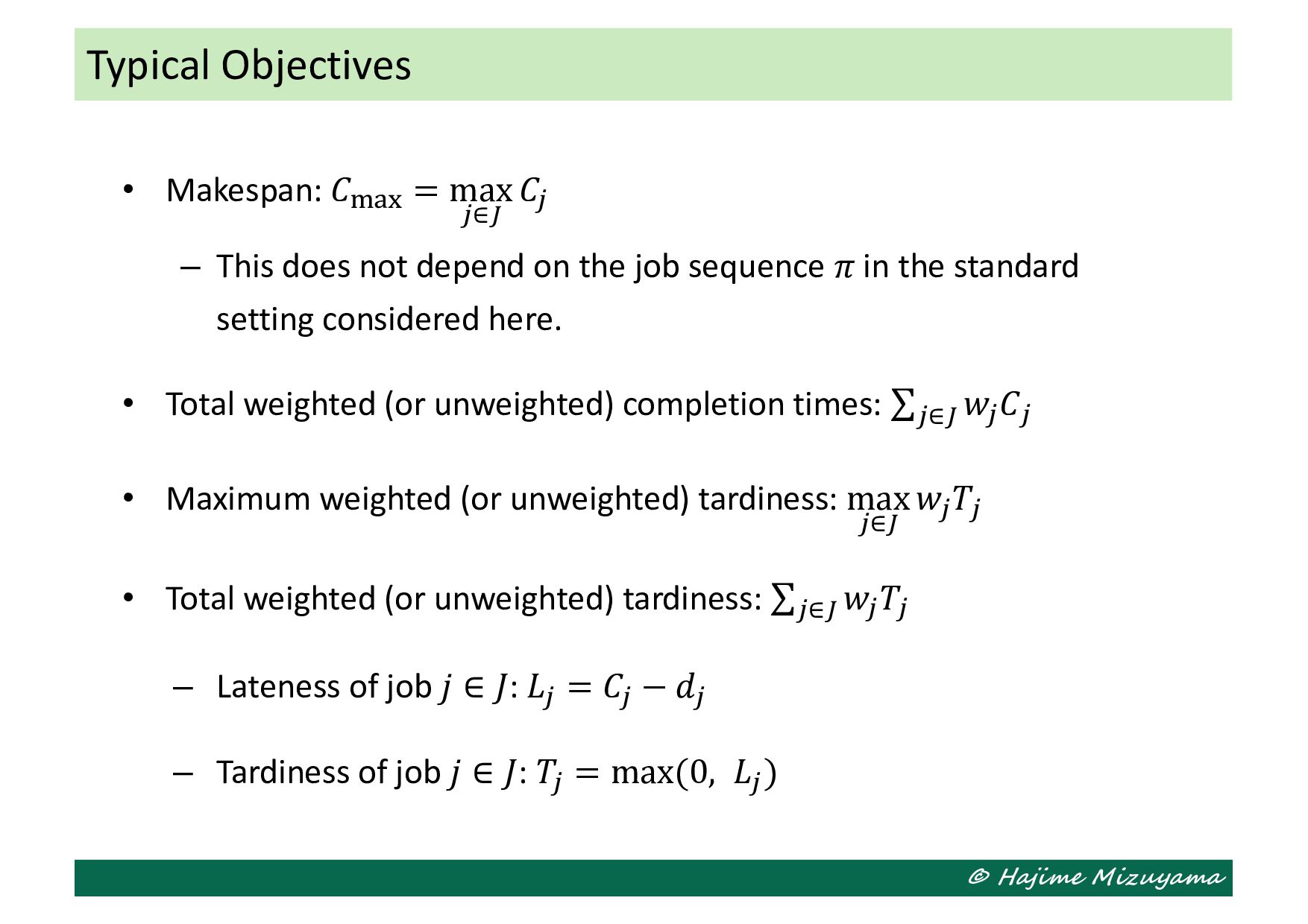
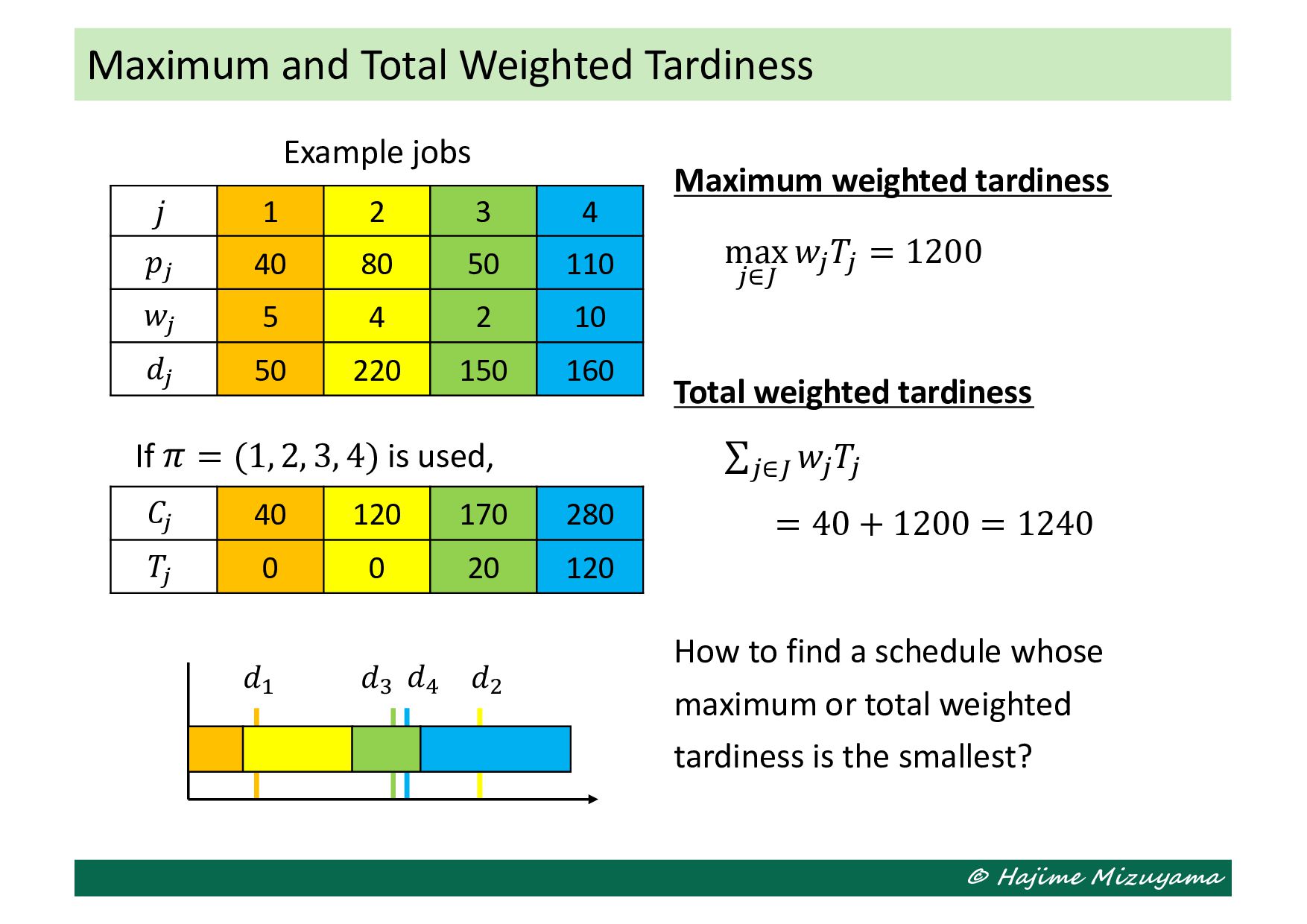
7. © Hajime Mizuyama • Makespan: 𝐶%&' = max !∈" 𝐶! – This does not depend on the job sequence 𝜋 in the standard setting considered here. • Total weighted (or unweighted) completion times: ∑!∈" 𝑤! 𝐶! • Maximum weighted (or unweighted) tardiness: max !∈" 𝑤! 𝑇! • Total weighted (or unweighted) tardiness: ∑!∈" 𝑤! 𝑇! – Lateness of job 𝑗 ∈ 𝐽: 𝐿! = 𝐶! − 𝑑! – Tardiness of job 𝑗 ∈ 𝐽: 𝑇! = max(0, 𝐿! ) Typical Objectives
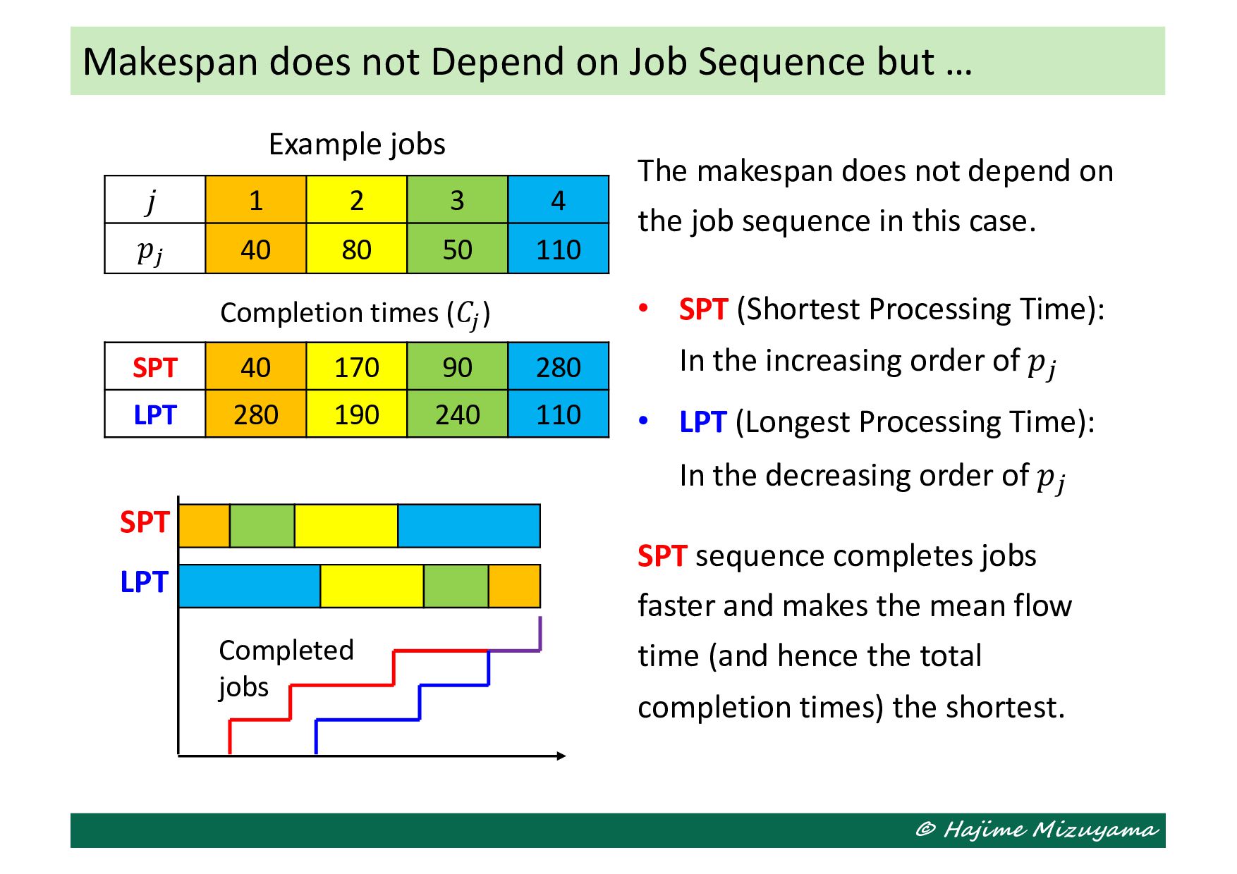
8. © Hajime Mizuyama Makespan does not Depend on Job Sequence but … 𝑗 1 2 3 4 𝑝! 40 80 50 110 SPT 40 170 90 280 LPT 280 190 240 110 The makespan does not depend on the job sequence in this case. • SPT (Shortest Processing Time): In the increasing order of 𝑝! • LPT (Longest Processing Time): In the decreasing order of 𝑝! SPT sequence completes jobs faster and makes the mean flow time (and hence the total completion times) the shortest. SPT LPT Completed jobs Completion times (𝐶! ) Example jobs
9. © Hajime Mizuyama Total Weighted Completion Times How to find a schedule whose total weighted completion times is the smallest? 𝑗 1 2 3 4 𝑝! 40 80 50 110 𝑤! 5 4 2 10 𝐶! 40 120 170 280 If 𝜋 = (1, 2, 3, 4) is used, ∑!∈" 𝑤! 𝐶! = 5×40 + 4×120 + 2×170 + 10×280 = 3820 𝑤! 𝐶! 𝜋 = (1, 2, 3, 4) Example jobs
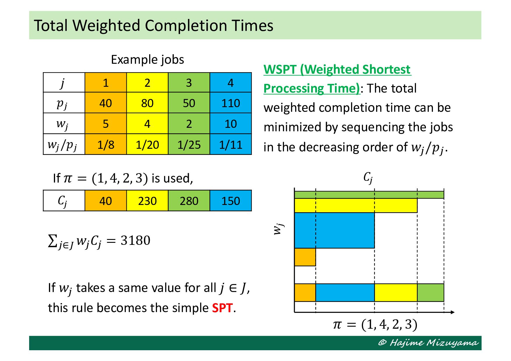
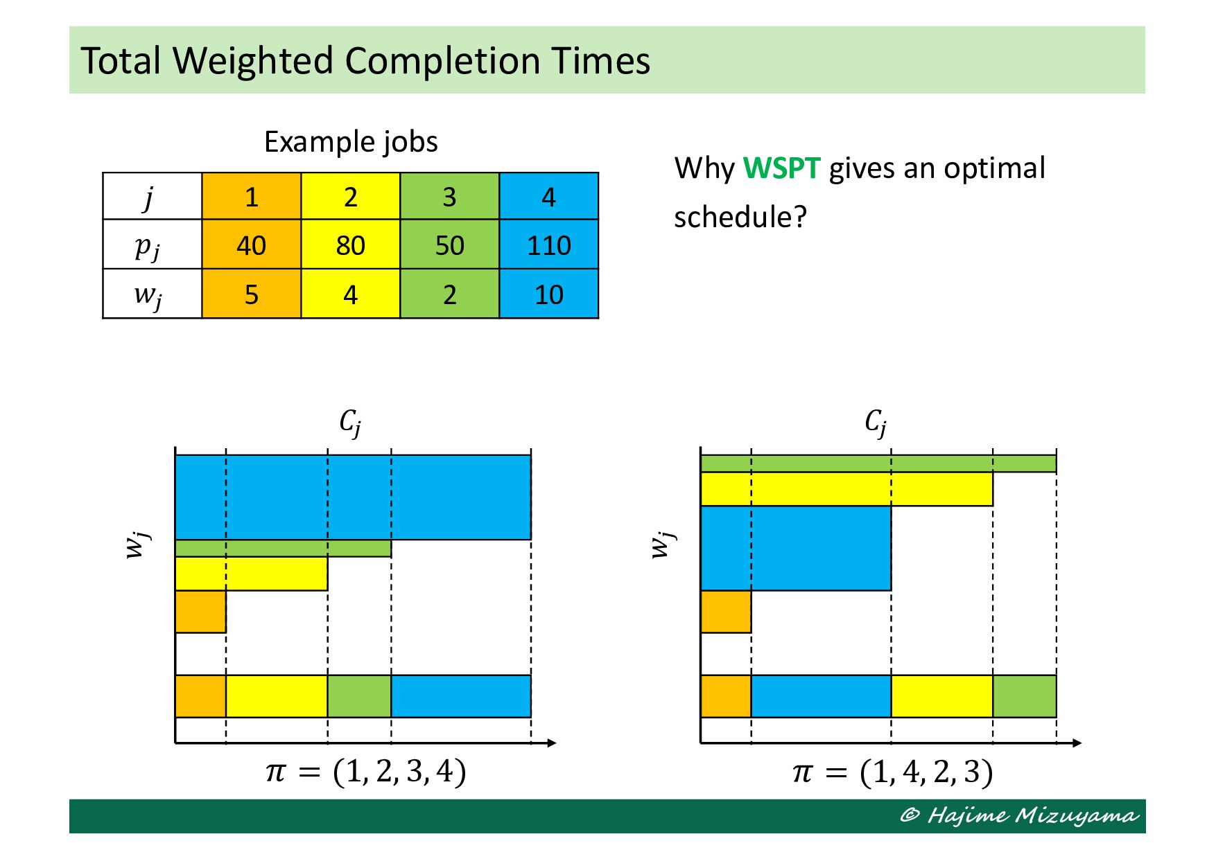
10. © Hajime Mizuyama 𝑤! 𝐶! Total Weighted Completion Times ∑!∈" 𝑤! 𝐶! = 3180 If 𝑤! takes a same value for all 𝑗 ∈ 𝐽, this rule becomes the simple SPT. WSPT (Weighted Shortest Processing Time): The total weighted completion time can be minimized by sequencing the jobs in the decreasing order of 𝑤! /𝑝!. 𝑗 1 2 3 4 𝑝! 40 80 50 110 𝑤! 5 4 2 10 𝑤! /𝑝! 1/8 1/20 1/25 1/11 𝐶! 40 230 280 150 𝜋 = (1, 4, 2, 3) If 𝜋 = (1, 4, 2, 3) is used, Example jobs
11. © Hajime Mizuyama Total Weighted Completion Times Why WSPT gives an optimal schedule? 𝑗 1 2 3 4 𝑝! 40 80 50 110 𝑤! 5 4 2 10 𝑤! 𝐶! 𝑤! 𝐶! 𝜋 = (1, 2, 3, 4) 𝜋 = (1, 4, 2, 3) Example jobs
12. © Hajime Mizuyama Maximum and Total Weighted Tardiness Maximum weighted tardiness max !∈" 𝑤! 𝑇! = 1200 Total weighted tardiness ∑!∈" 𝑤! 𝑇! = 40 + 1200 = 1240 How to find a schedule whose maximum or total weighted tardiness is the smallest? 𝑗 1 2 3 4 𝑝! 40 80 50 110 𝑤! 5 4 2 10 𝑑! 50 220 150 160 𝐶! 40 120 170 280 𝑇 ! 0 0 20 120 𝑑" 𝑑# 𝑑$ 𝑑% If 𝜋 = (1, 2, 3, 4) is used, Example jobs
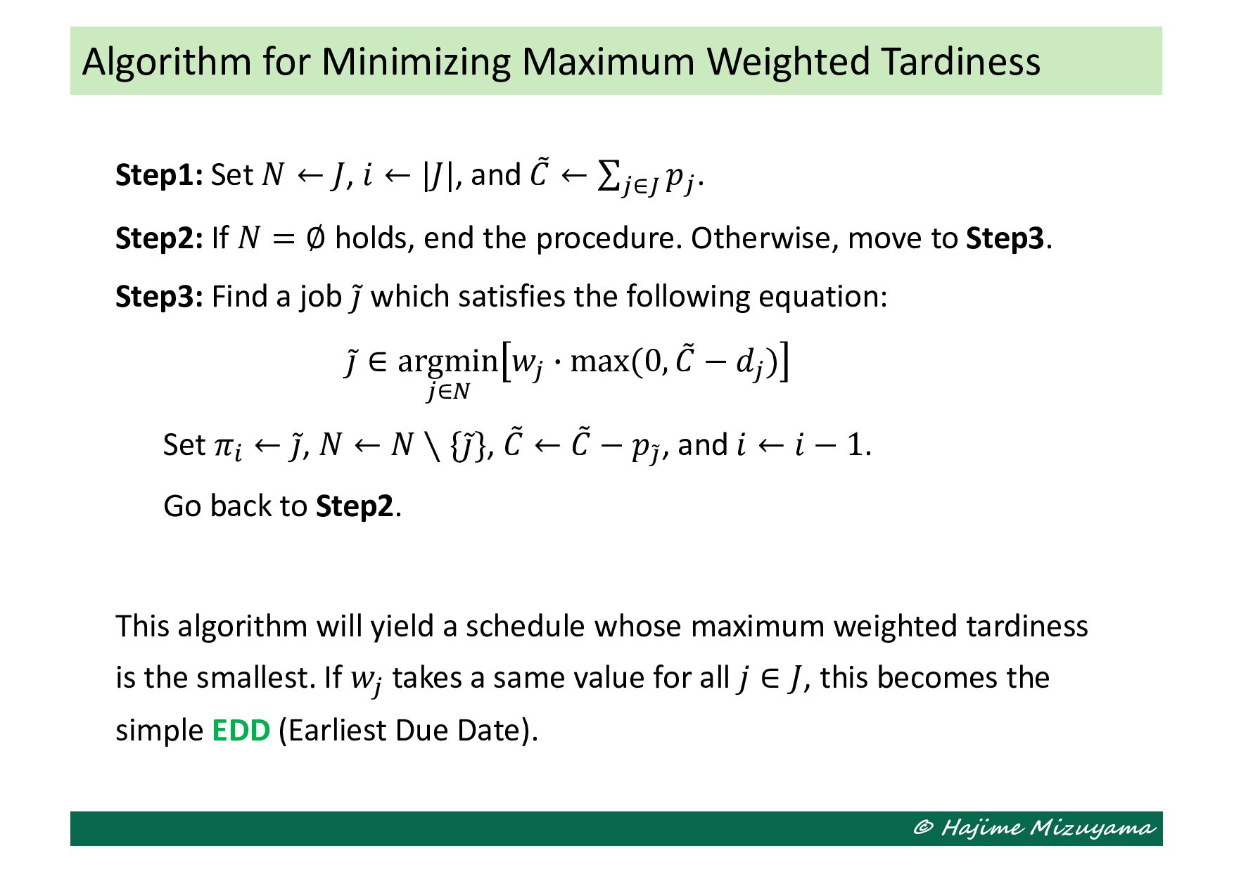
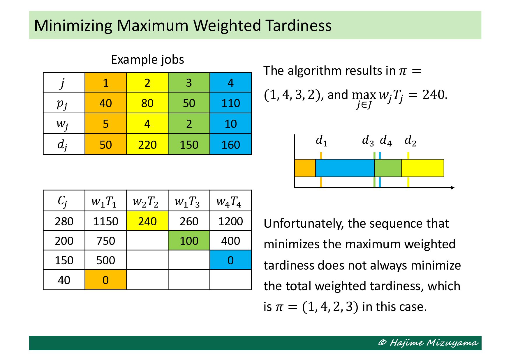
13. © Hajime Mizuyama Step1: Set 𝑁 ← 𝐽, 𝑖 ← |𝐽|, and I 𝐶 ← ∑!∈" 𝑝!. Step2: If 𝑁 = ∅ holds, end the procedure. Otherwise, move to Step3. Step3: Find a job ̃ 𝚥 which satisfies the following equation: ̃ 𝚥 ∈ argmin !∈) 𝑤! Q max(0, I 𝐶 − 𝑑! ) Set 𝜋* ← ̃ 𝚥, 𝑁 ← 𝑁 ∖ { ̃ 𝚥}, I 𝐶 ← I 𝐶 − 𝑝 ̃ ,, and 𝑖 ← 𝑖 − 1. Go back to Step2. This algorithm will yield a schedule whose maximum weighted tardiness is the smallest. If 𝑤! takes a same value for all 𝑗 ∈ 𝐽, this becomes the simple EDD (Earliest Due Date). Algorithm for Minimizing Maximum Weighted Tardiness
14. © Hajime Mizuyama 𝑑" 𝑑# 𝑑$ 𝑑% Minimizing Maximum Weighted Tardiness The algorithm results in 𝜋 = (1, 4, 3, 2), and max !∈" 𝑤! 𝑇! = 240. Unfortunately, the sequence that minimizes the maximum weighted tardiness does not always minimize the total weighted tardiness, which is 𝜋 = (1, 4, 2, 3) in this case. 𝑗 1 2 3 4 𝑝! 40 80 50 110 𝑤! 5 4 2 10 𝑑! 50 220 150 160 𝐶! 𝑤" 𝑇" 𝑤# 𝑇# 𝑤" 𝑇$ 𝑤% 𝑇% 280 1150 240 260 1200 200 750 100 400 150 500 0 40 0 Example jobs
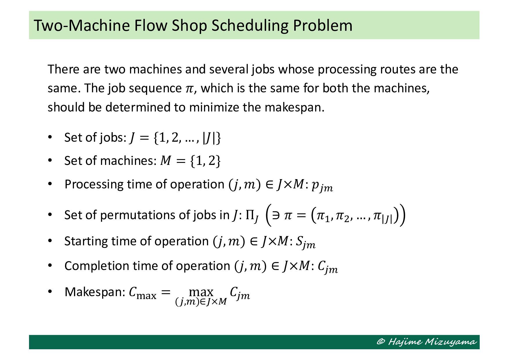
15. © Hajime Mizuyama There are two machines and several jobs whose processing routes are the same. The job sequence 𝜋, which is the same for both the machines, should be determined to minimize the makespan. • Set of jobs: 𝐽 = {1, 2, … , |𝐽|} • Set of machines: 𝑀 = {1, 2} • Processing time of operation (𝑗, 𝑚) ∈ 𝐽×𝑀: 𝑝!- • Set of permutations of jobs in 𝐽: Π" ∋ 𝜋 = 𝜋# , 𝜋$ , … , 𝜋 " • Starting time of operation (𝑗, 𝑚) ∈ 𝐽×𝑀: 𝑆!- • Completion time of operation (𝑗, 𝑚) ∈ 𝐽×𝑀: 𝐶!- • Makespan: 𝐶%&' = max (!,-)∈"×2 𝐶!- Two-Machine Flow Shop Scheduling Problem
16. © Hajime Mizuyama Illustrative Example: Two-Machine Flow Shop Interference between machines results in waiting times. M2 cannot start processing a job until M1 completes the job. M1 M2 𝑗 1 2 3 4 𝑝!" 40 80 50 110 𝑝!# 120 30 80 50 Example jobs If 𝜋 = (1, 2, 3, 4) is used, then …
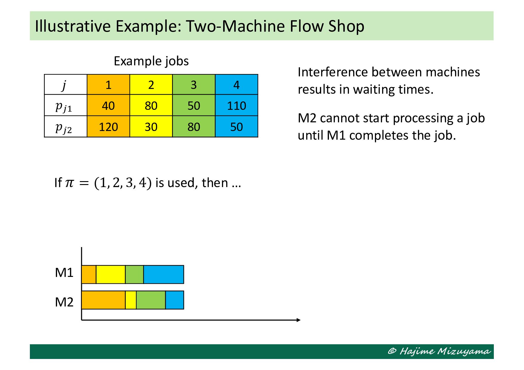
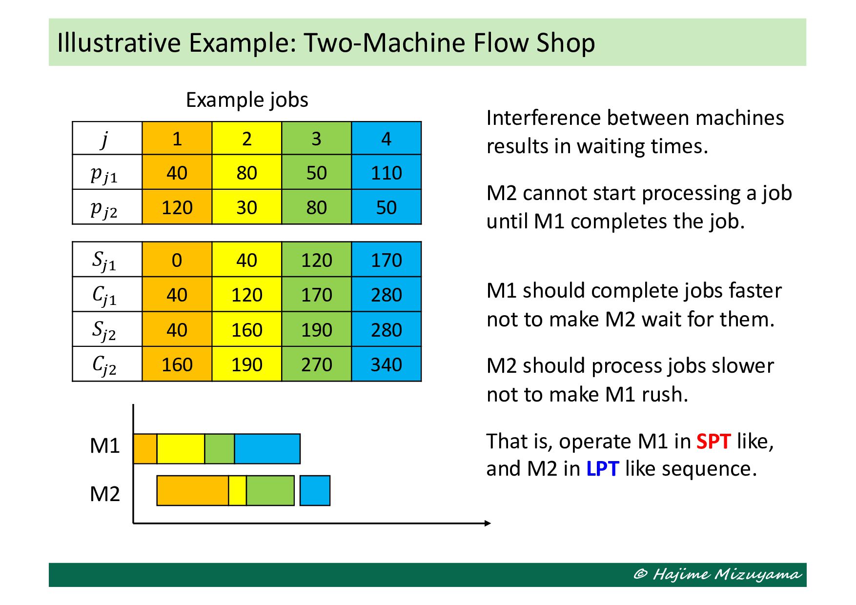
17. © Hajime Mizuyama Illustrative Example: Two-Machine Flow Shop M1 should complete jobs faster not to make M2 wait for them. M2 should process jobs slower not to make M1 rush. That is, operate M1 in SPT like, and M2 in LPT like sequence. Interference between machines results in waiting times. M2 cannot start processing a job until M1 completes the job. Example jobs M1 M2 𝑗 1 2 3 4 𝑝!" 40 80 50 110 𝑝!# 120 30 80 50 𝑆!" 0 40 120 170 𝐶!" 40 120 170 280 𝑆!# 40 160 190 280 𝐶!# 160 190 270 340
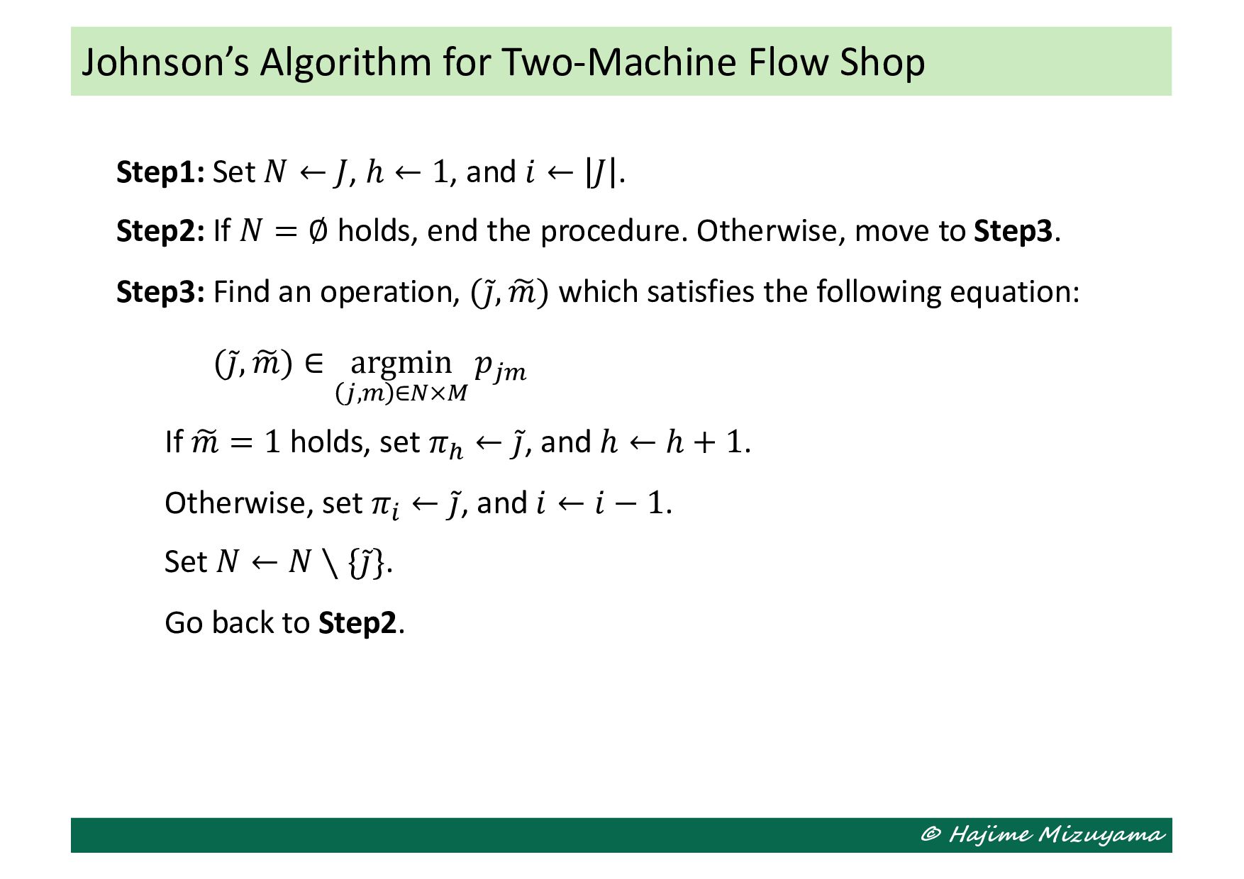
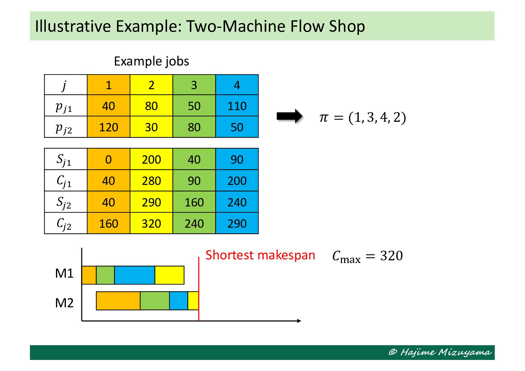
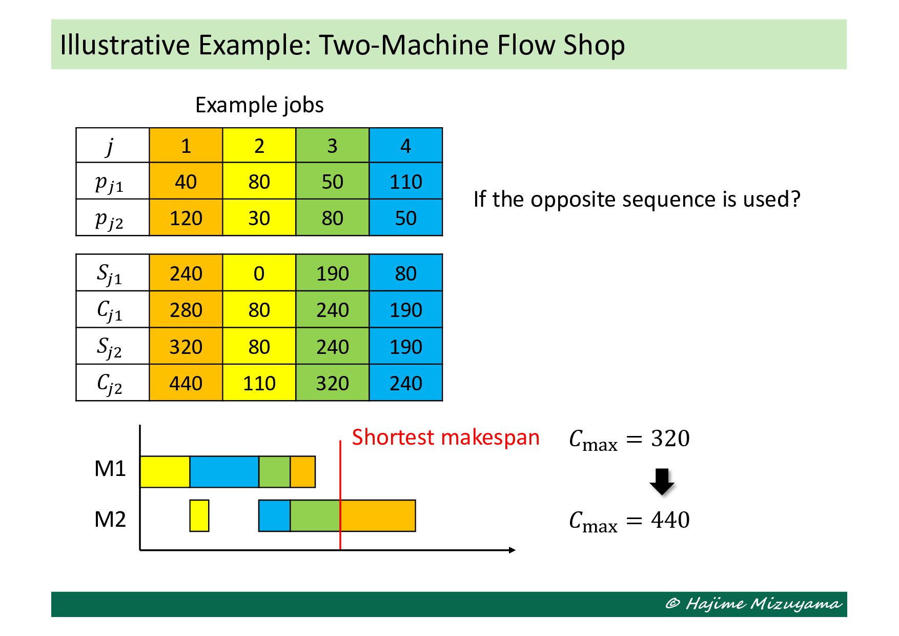
18. © Hajime Mizuyama Step1: Set 𝑁 ← 𝐽, ℎ ← 1, and 𝑖 ← 𝐽 . Step2: If 𝑁 = ∅ holds, end the procedure. Otherwise, move to Step3. Step3: Find an operation, ( ̃ 𝚥, W 𝑚) which satisfies the following equation: ( ̃ 𝚥, W 𝑚) ∈ argmin !,- ∈)×2 𝑝!- If W 𝑚 = 1 holds, set 𝜋3 ← ̃ 𝚥, and ℎ ← ℎ + 1. Otherwise, set 𝜋* ← ̃ 𝚥, and 𝑖 ← 𝑖 − 1. Set 𝑁 ← 𝑁 ∖ { ̃ 𝚥}. Go back to Step2. Johnson’s Algorithm for Two-Machine Flow Shop
19. © Hajime Mizuyama Illustrative Example: Two-Machine Flow Shop Example jobs M1 M2 Shortest makespan 𝑗 1 2 3 4 𝑝!" 40 80 50 110 𝑝!# 120 30 80 50 𝑆!" 0 200 40 90 𝐶!" 40 280 90 200 𝑆!# 40 290 160 240 𝐶!# 160 320 240 290 𝜋 = (1, 3, 4, 2) 𝐶%&' = 320
20. © Hajime Mizuyama Illustrative Example: Two-Machine Flow Shop Shortest makespan Example jobs M1 M2 If the opposite sequence is used? 𝑗 1 2 3 4 𝑝!" 40 80 50 110 𝑝!# 120 30 80 50 𝑆!" 240 0 190 80 𝐶!" 280 80 240 190 𝑆!# 320 80 240 190 𝐶!# 440 110 320 240 𝐶%&' = 440 𝐶%&' = 320
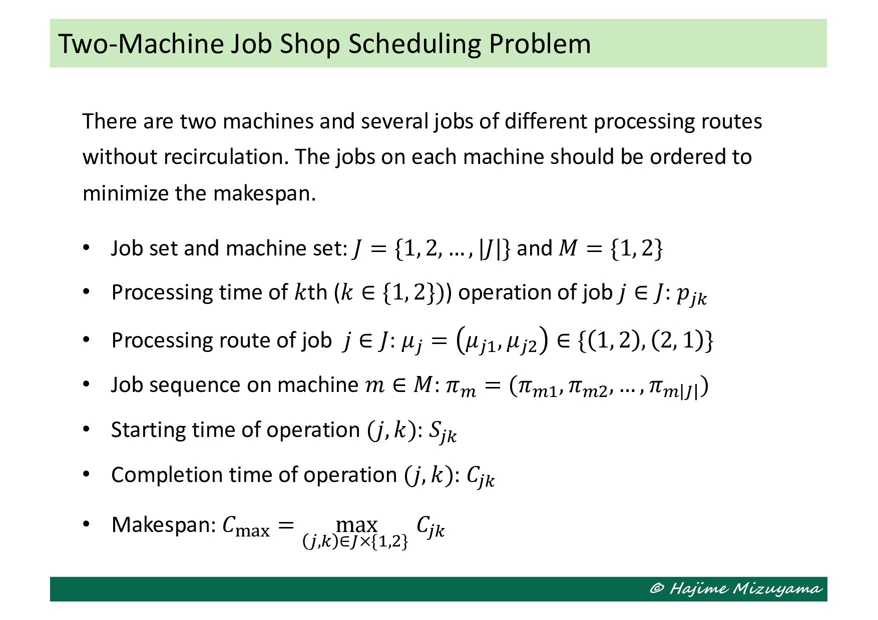
21. © Hajime Mizuyama There are two machines and several jobs of different processing routes without recirculation. The jobs on each machine should be ordered to minimize the makespan. • Job set and machine set: 𝐽 = {1, 2, … , |𝐽|} and 𝑀 = {1, 2} • Processing time of 𝑘th (𝑘 ∈ {1, 2})) operation of job 𝑗 ∈ 𝐽: 𝑝!4 • Processing route of job 𝑗 ∈ 𝐽: 𝜇! = 𝜇!# , 𝜇!$ ∈ { 1, 2 , 2, 1 } • Job sequence on machine 𝑚 ∈ 𝑀: 𝜋- = (𝜋-# , 𝜋-$ , … , 𝜋- " ) • Starting time of operation (𝑗, 𝑘): 𝑆!4 • Completion time of operation (𝑗, 𝑘): 𝐶!4 • Makespan: 𝐶%&' = max !,4 ∈"×{#,$} 𝐶!4 Two-Machine Job Shop Scheduling Problem
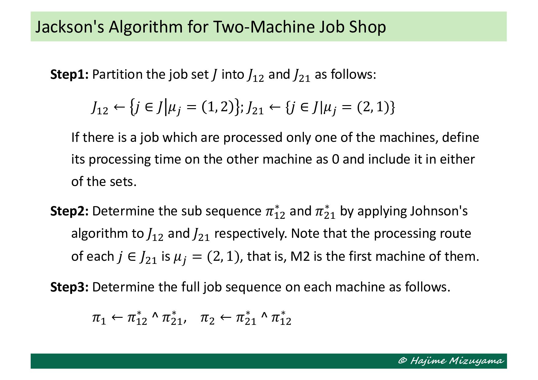
22. © Hajime Mizuyama Step1: Partition the job set 𝐽 into 𝐽#$ and 𝐽$# as follows: 𝐽#$ ← 𝑗 ∈ 𝐽 𝜇! = 1, 2 ; 𝐽$# ← {𝑗 ∈ 𝐽|𝜇! = (2, 1)} If there is a job which are processed only one of the machines, define its processing time on the other machine as 0 and include it in either of the sets. Step2: Determine the sub sequence 𝜋#$ ∗ and 𝜋$# ∗ by applying Johnson's algorithm to 𝐽#$ and 𝐽$# respectively. Note that the processing route of each 𝑗 ∈ 𝐽$# is 𝜇! = (2, 1), that is, M2 is the first machine of them. Step3: Determine the full job sequence on each machine as follows. 𝜋# ← 𝜋#$ ∗ ^ 𝜋$# ∗ , 𝜋$ ← 𝜋$# ∗ ^ 𝜋#$ ∗ Jackson's Algorithm for Two-Machine Job Shop
23. © Hajime Mizuyama 𝑘 = 1 𝑘 = 2 𝜇!" 𝑝!" 𝜇!# 𝑝!" 𝑗 = 1 M1 10 M2 25 𝑗 = 2 M1 40 M2 15 𝑗 = 3 M1 25 M2 50 𝑗 = 4 M1 20 M2 0 𝑗 = 5 M2 30 M1 45 𝑗 = 6 M2 15 M1 20 𝑗 = 7 M2 35 M1 25 Illustrative Example: Two-Machine Job Shop 𝜋#$ ∗ = (1, 3, 2, 4) 𝜋$# ∗ = (6, 5, 7) 𝜋# = (1, 3, 2, 4, 6, 5, 7) 𝜋$ = (6, 5, 7, 1, 3, 2)
24. © Hajime Mizuyama Illustrative Example: Two-Machine Job Shop M1 M2 3 1 2 5 4 7 6 3 1 2 5 7 6 𝐶%&' = 185 𝜋#$ ∗ = (1, 3, 2, 4) 𝜋$# ∗ = (6, 5, 7) 𝜋# = (1, 3, 2, 4, 6, 5, 7) 𝜋$ = (6, 5, 7, 1, 3, 2)