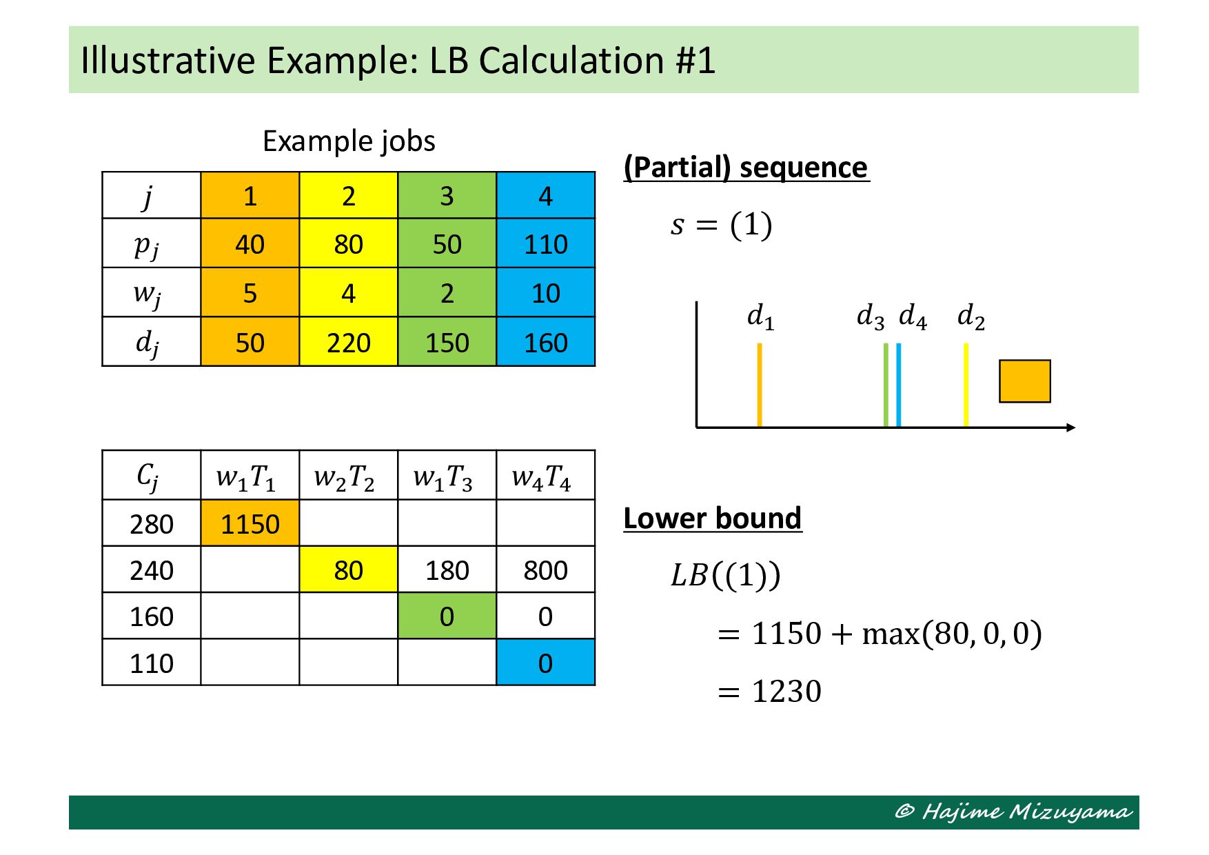
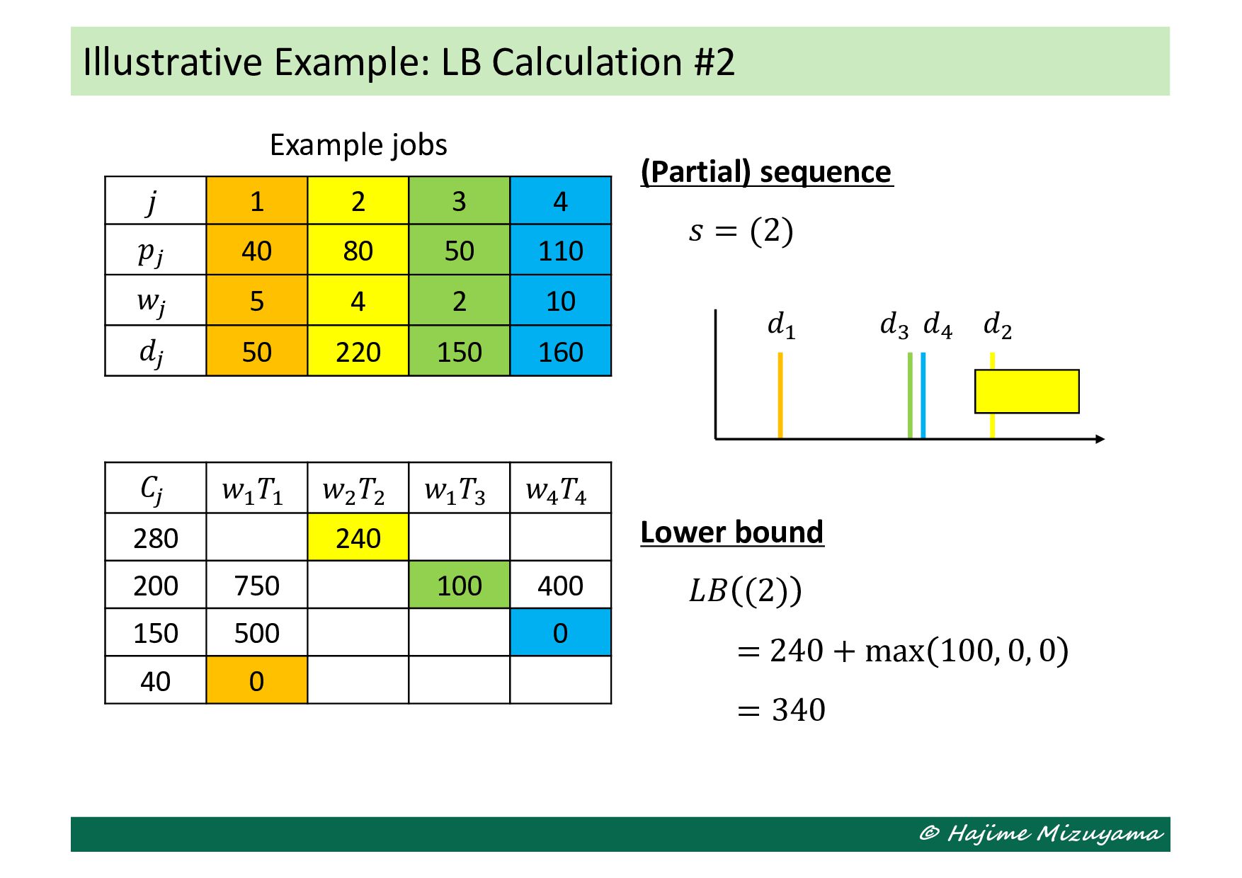
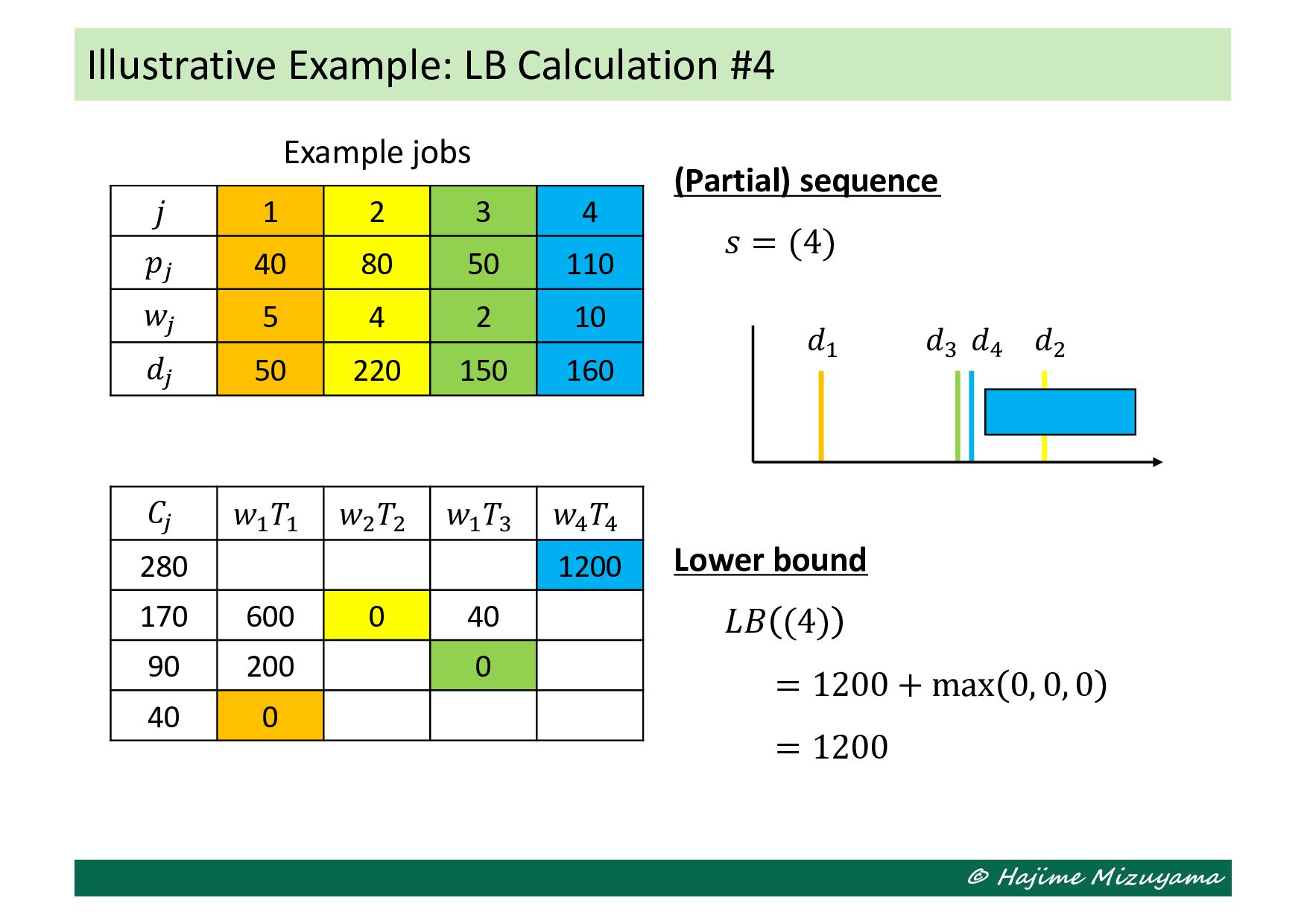
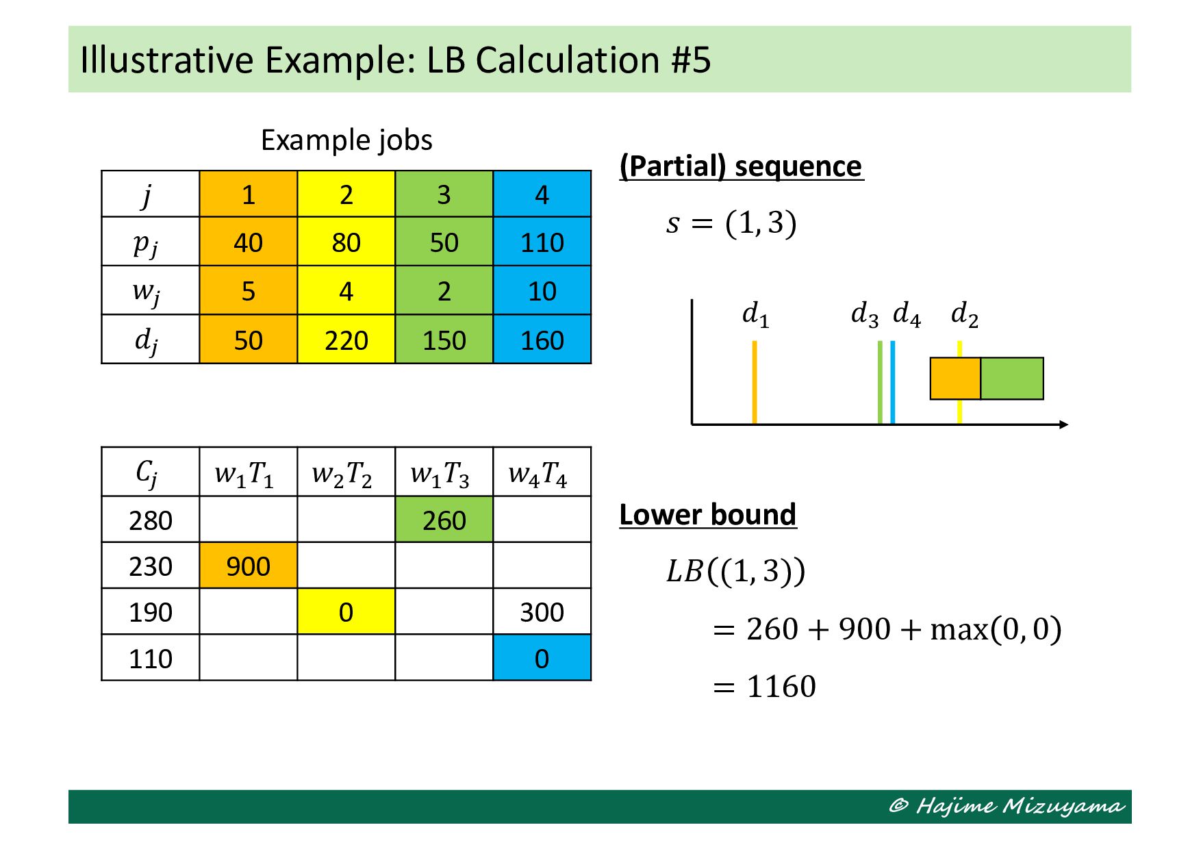
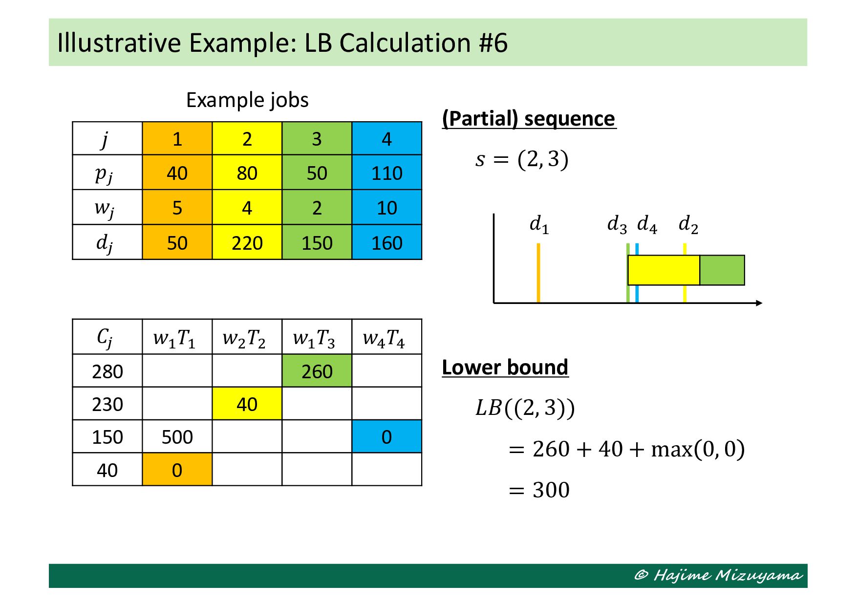
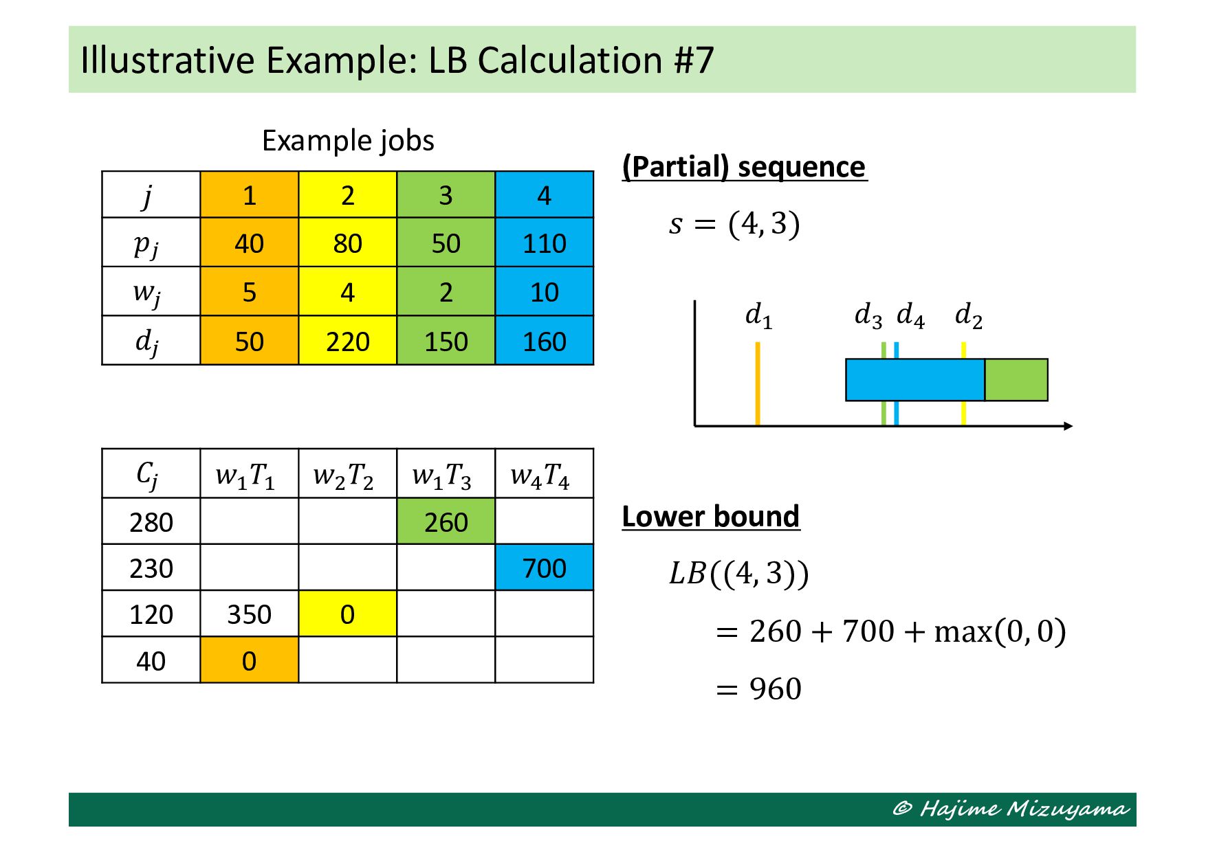
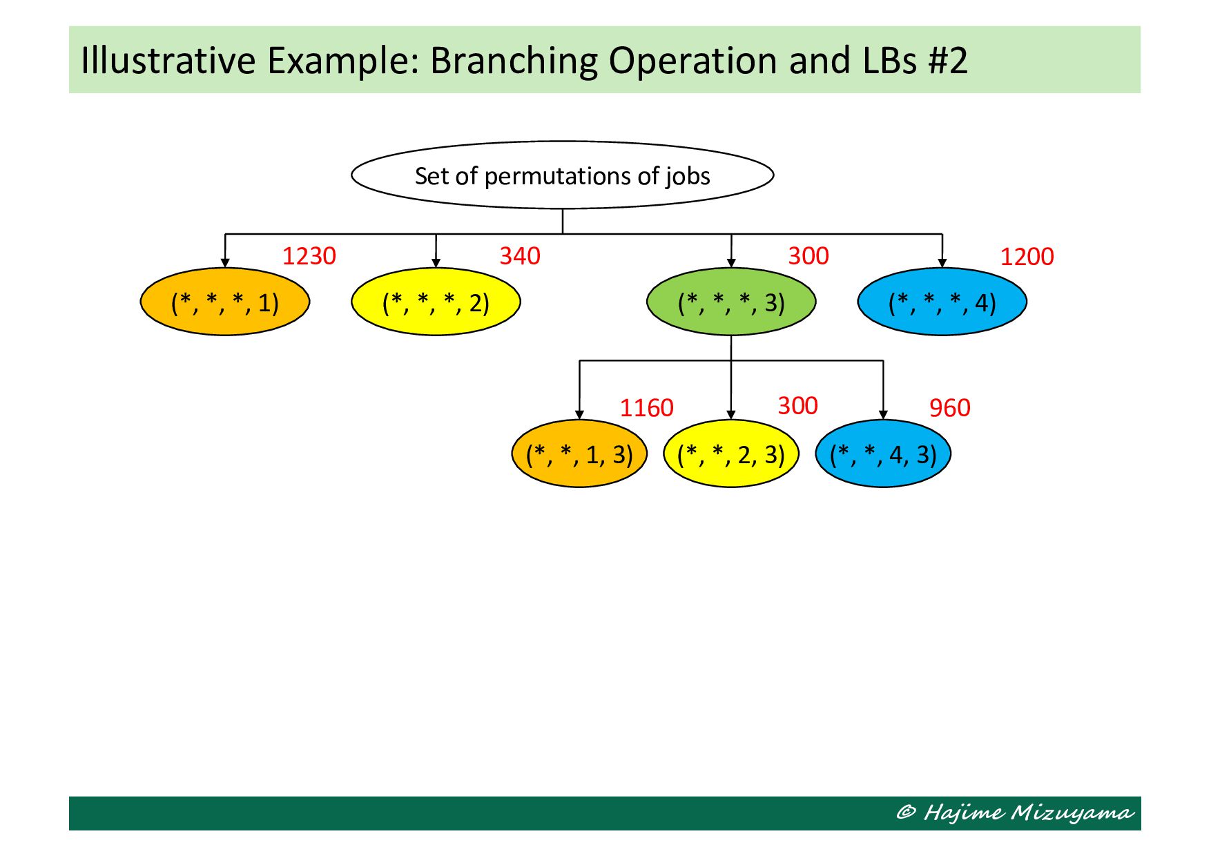
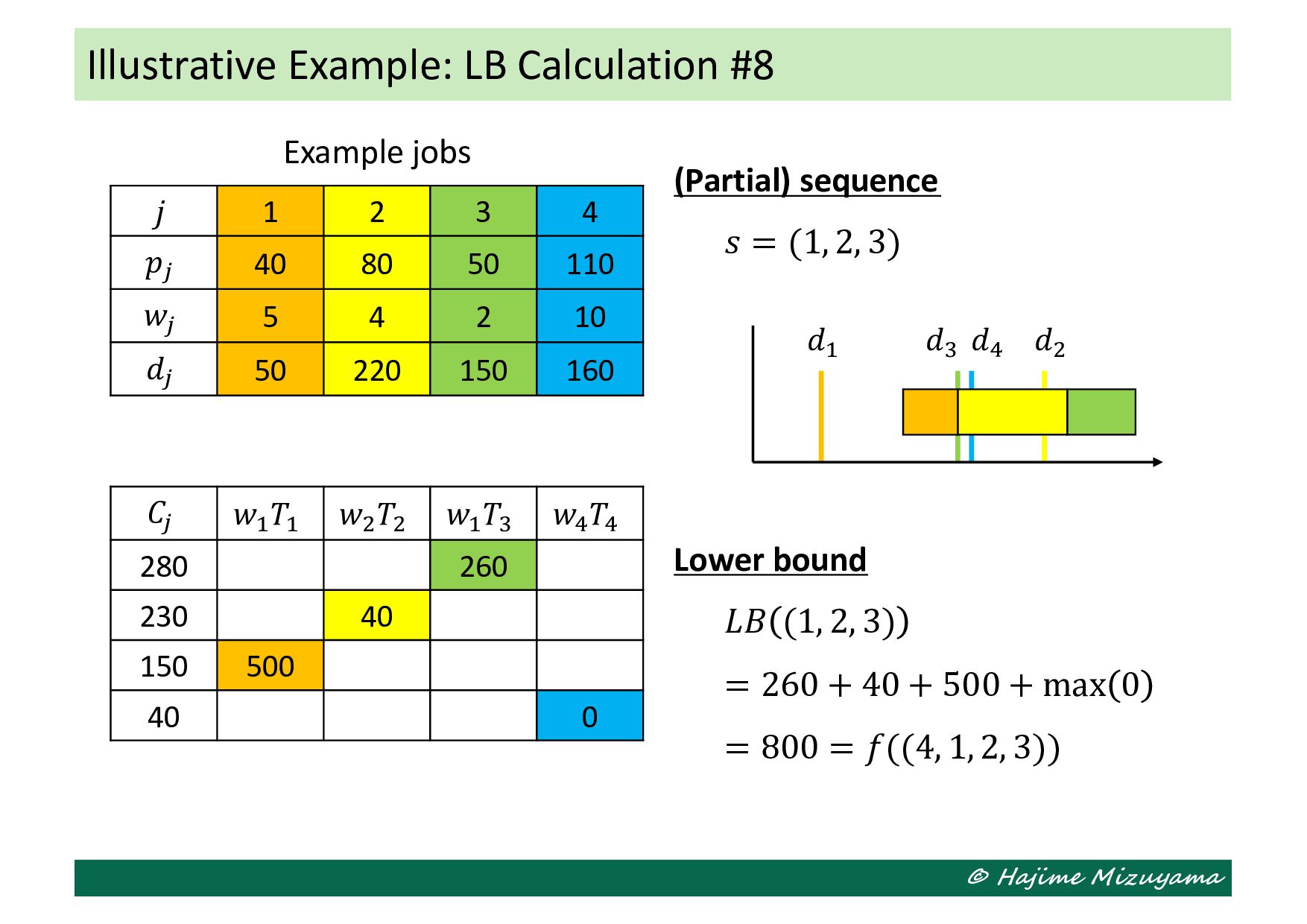
Upgrade to Pro — share decks privately, control downloads, hide ads and more …

Lecture slides for POM 2-3

hajimizu
September 08, 2023

Lecture slides for POM 2-3

生産管理技術2の講義3のスライドです.

hajimizu

September 08, 2023
Tweet

More Decks by hajimizu

Other Decks in Technology

Transcript

  1. © Hajime Mizuyama Production & Operations Management #2 @AGU Lec.3:

    Single Machine Scheduling #2 • Minimizing total weighted tardiness (revisited) • Enumerating all permutations of jobs • Branch and bound (BAB)
  2. © Hajime Mizuyama Course Schedule #1 Date Contents Single machine

    scheduling (1): Dynamic programming (DP) Single machine scheduling (2): Branch and bound (BAB) Flow shop scheduling: Unlimited, limited, and no buffer capacity cases, and branch and bound (BAB) Metaheuristics: Local search, simulated annealing, tabu search, genetic algorithm, etc. Job shop scheduling (1): Disjunctive graph representation, and 0-1 mixed-integer linear programming (0-1 MILP) formulation Job shop scheduling (2): How to enumerate active schedules, and branch and bound (BAB) Mid-term examination
  3. © Hajime Mizuyama There are only one machine and several

    jobs. The sequence of the jobs 𝜋 should be properly determined to minimize total weighted tardiness. • Set of jobs: 𝐽 = {1, 2, … , |𝐽|} • Processing time of job 𝑗 ∈ 𝐽: 𝑝! • Weight of job 𝑗 ∈ 𝐽: 𝑤! • Due date of job 𝑗 ∈ 𝐽: 𝑑! • Set of permutations of jobs in 𝐽: Π" ∋ 𝜋 = 𝜋# , 𝜋$ , … , 𝜋 " • Starting time of job 𝑗 ∈ 𝐽: 𝑆! • Completion time of job 𝑗 ∈ 𝐽: 𝐶! • Objective function: 𝑓 𝜋 = ∑!∈" 𝑤! 𝑇! = ∑!∈" 𝑤! max(0, 𝐶! − 𝑑! ) Sigle-Machine Scheduling Problem to Minimize Total Weighted Tardiness
  4. © Hajime Mizuyama Set of permutations of jobs Set of

    permutations of jobs (*, *, *, 1) (*, *, *, 2) 3! (*, *, *, 4) (*, *, *, 3) (*, *, *, 2) (*, *, *, 1) (*, *, 4, 1) (*, *, 3, 1) (*, *, 2, 1) (*, *, 4, 1) Branching and Search Tree (|J|=4) 4! 2! (*, *, 4, 2) (*, *, 3, 2) (*, *, 1, 2) 1! (3, 2, 4, 1) (2, 3, 4, 1)
  5. © Hajime Mizuyama • Each intermediate node of the search

    tree corresponds to a subset of possible permutations of jobs (or proper job sequences). • If a lower bound (LB) can be specified to an intermediate node, we can tell that the node does not contain any job sequence whose objective function value is smaller than the LB. • This means that, if we have already found a temporary solution whose objective function value is smaller than the LB, we do not need to evaluate the job sequences in the node. • It is called bounding operation to remove the unsplit nodes having a LB inferior to the temporary solution’s objective function value (UB). • The LB values can also be used to determine which node to branch next (e.g., choosing the one with the smallest LB). Lower Bound (LB) and Bounding
  6. © Hajime Mizuyama BAB Algorithm for Minimizing Total Weighted Tardiness

    𝑁 ← {∅}; 𝑈𝐵 ← ∞; 𝜋 ← ∅ while 𝑁 ≠ ∅ do Choose 𝑠 = (𝑠# , 𝑠$ , … ) ∈ 𝑁 𝑁 ← 𝑁 ∖ {𝑠} for 𝑗 ∈ 𝐽 ∖ 𝑠 do ̃ 𝑠 ← 𝑗 ^ 𝑠 Calculate 𝐿𝐵( ̃ 𝑠) if 𝐿𝐵 ̃ 𝑠 < 𝑈𝐵 then if 𝐽 ∖ ̃ 𝑠 = ∅ then 𝑈𝐵 ← 𝐿𝐵( ̃ 𝑠) 𝜋 ← ̃ 𝑠 𝑁 ← 𝜎 ∈ 𝑁 𝐿𝐵(𝜎) < 𝑈𝐵} else 𝑁 ← 𝑁 ∪ { ̃ 𝑠} fi fi od od
  7. © Hajime Mizuyama For each (partial) sequence 𝑠 (specified from

    the tail), we can assign the set of full sequences which accords with the given 𝑠 as: L Π" (𝑠) = 𝜋 ∈ Π" (𝜋 " & ' (# , … , 𝜋 " ) = 𝑠} Any lower bound 𝐿𝐵(𝑠) corresponding to the sequence should satisfy: 𝐿𝐵 𝑠 ≤ min )∈* +(') 𝑓 𝜋 = min )∈* +(') ∑!∈" 𝑤! 𝑇! 𝑇! for each 𝑗 ∈ 𝑠 and min )∈* +!(') max !∈"∖' 𝑤! 𝑇! for the set of unassigned jobs can be evaluated without specifying the rest of the sequence. Hence, 𝐿𝐵 𝑠 = ∑!∈' 𝑤! 𝑇! + min )∈* +!(') max !∈"∖' 𝑤! 𝑇! can be used as the lower bound. Lower Bound (LB) for Total Weighted Tardiness
  8. © Hajime Mizuyama 𝑑! 𝑑" 𝑑# 𝑑$ Illustrative Example: LB

    Calculation #1 (Partial) sequence 𝑠 = (1) Lower bound 𝐿𝐵 (1) = 1150 + max 80, 0, 0 = 1230 𝑗 1 2 3 4 𝑝% 40 80 50 110 𝑤% 5 4 2 10 𝑑% 50 220 150 160 𝐶% 𝑤! 𝑇! 𝑤" 𝑇" 𝑤! 𝑇# 𝑤$ 𝑇$ 280 1150 240 80 180 800 160 0 0 110 0 Example jobs
  9. © Hajime Mizuyama 𝑑! 𝑑" 𝑑# 𝑑$ Illustrative Example: LB

    Calculation #2 (Partial) sequence 𝑠 = (2) Lower bound 𝐿𝐵 (2) = 240 + max 100, 0, 0 = 340 𝑗 1 2 3 4 𝑝% 40 80 50 110 𝑤% 5 4 2 10 𝑑% 50 220 150 160 𝐶% 𝑤! 𝑇! 𝑤" 𝑇" 𝑤! 𝑇# 𝑤$ 𝑇$ 280 240 200 750 100 400 150 500 0 40 0 Example jobs
  10. © Hajime Mizuyama 𝑑! 𝑑" 𝑑# 𝑑$ Illustrative Example: LB

    Calculation #3 (Partial) sequence 𝑠 = (3) Lower bound 𝐿𝐵 (3) = 260 + max 40, 0, 0 = 300 𝑗 1 2 3 4 𝑝% 40 80 50 110 𝑤% 5 4 2 10 𝑑% 50 220 150 160 𝐶% 𝑤! 𝑇! 𝑤" 𝑇" 𝑤! 𝑇# 𝑤$ 𝑇$ 280 260 230 900 40 700 150 500 0 40 0 Example jobs
  11. © Hajime Mizuyama 𝑑! 𝑑" 𝑑# 𝑑$ Illustrative Example: LB

    Calculation #4 (Partial) sequence 𝑠 = (4) Lower bound 𝐿𝐵 (4) = 1200 + max 0, 0, 0 = 1200 𝑗 1 2 3 4 𝑝% 40 80 50 110 𝑤% 5 4 2 10 𝑑% 50 220 150 160 𝐶% 𝑤! 𝑇! 𝑤" 𝑇" 𝑤! 𝑇# 𝑤$ 𝑇$ 280 1200 170 600 0 40 90 200 0 40 0 Example jobs
  12. © Hajime Mizuyama Set of permutations of jobs Illustrative Example:

    Branching Operation and LBs #1 (*, *, *, 1) (*, *, *, 2) (*, *, *, 4) (*, *, *, 3) 1200 300 340 1230
  13. © Hajime Mizuyama 𝑑! 𝑑" 𝑑# 𝑑$ Illustrative Example: LB

    Calculation #5 (Partial) sequence 𝑠 = (1, 3) Lower bound 𝐿𝐵 (1, 3) = 260 + 900 + max 0, 0 = 1160 𝑗 1 2 3 4 𝑝% 40 80 50 110 𝑤% 5 4 2 10 𝑑% 50 220 150 160 𝐶% 𝑤! 𝑇! 𝑤" 𝑇" 𝑤! 𝑇# 𝑤$ 𝑇$ 280 260 230 900 190 0 300 110 0 Example jobs
  14. © Hajime Mizuyama 𝑑! 𝑑" 𝑑# 𝑑$ Illustrative Example: LB

    Calculation #6 (Partial) sequence 𝑠 = (2, 3) Lower bound 𝐿𝐵((2, 3)) = 260 + 40 + max 0, 0 = 300 𝑗 1 2 3 4 𝑝% 40 80 50 110 𝑤% 5 4 2 10 𝑑% 50 220 150 160 𝐶% 𝑤! 𝑇! 𝑤" 𝑇" 𝑤! 𝑇# 𝑤$ 𝑇$ 280 260 230 40 150 500 0 40 0 Example jobs
  15. © Hajime Mizuyama 𝑑! 𝑑" 𝑑# 𝑑$ Illustrative Example: LB

    Calculation #7 (Partial) sequence 𝑠 = (4, 3) Lower bound 𝐿𝐵((4, 3)) = 260 + 700 + max 0, 0 = 960 𝑗 1 2 3 4 𝑝% 40 80 50 110 𝑤% 5 4 2 10 𝑑% 50 220 150 160 𝐶% 𝑤! 𝑇! 𝑤" 𝑇" 𝑤! 𝑇# 𝑤$ 𝑇$ 280 260 230 700 120 350 0 40 0 Example jobs
  16. © Hajime Mizuyama Set of permutations of jobs Illustrative Example:

    Branching Operation and LBs #2 (*, *, *, 1) (*, *, *, 2) (*, *, *, 4) (*, *, *, 3) 1200 300 340 1230 (*, *, 4, 3) (*, *, 2, 3) (*, *, 1, 3) 1160 300 960
  17. © Hajime Mizuyama 𝑑! 𝑑" 𝑑# 𝑑$ Illustrative Example: LB

    Calculation #8 (Partial) sequence 𝑠 = (1, 2, 3) Lower bound 𝐿𝐵 (1, 2, 3) = 260 + 40 + 500 + max 0 = 800 = 𝑓((4, 1, 2, 3)) 𝑗 1 2 3 4 𝑝% 40 80 50 110 𝑤% 5 4 2 10 𝑑% 50 220 150 160 𝐶% 𝑤! 𝑇! 𝑤" 𝑇" 𝑤! 𝑇# 𝑤$ 𝑇$ 280 260 230 40 150 500 40 0 Example jobs
  18. © Hajime Mizuyama 𝑑! 𝑑" 𝑑# 𝑑$ Illustrative Example: LB

    Calculation #9 (Partial) sequence 𝑠 = (4, 2, 3) Lower bound 𝐿𝐵 (4, 2, 3) = 260 + 40 + 0 + max 0 = 300 = 𝑓((1, 4, 2, 3)) 𝑗 1 2 3 4 𝑝% 40 80 50 110 𝑤% 5 4 2 10 𝑑% 50 220 150 160 𝐶% 𝑤! 𝑇! 𝑤" 𝑇" 𝑤! 𝑇# 𝑤$ 𝑇$ 280 260 230 40 150 0 40 0 Example jobs
  19. © Hajime Mizuyama Set of permutations of jobs Illustrative Example:

    Bounding Operation #1 (*, *, *, 1) (*, *, *, 2) (*, *, *, 4) (*, *, *, 3) 1200 300 340 1230 (*, *, 4, 3) (*, *, 2, 3) (*, *, 1, 3) 1160 300 960 (1, 4, 2, 3) (4, 1, 2, 3) 800 300
  20. © Hajime Mizuyama Set of permutations of jobs Illustrative Example:

    Bounding Operation #2 (*, *, *, 1) (*, *, *, 2) (*, *, *, 4) (*, *, *, 3) 1200 300 340 1230 (*, *, 4, 3) (*, *, 2, 3) (*, *, 1, 3) 1160 300 960 (1, 4, 2, 3) (4, 1, 2, 3) 800 300