Lecture slides for POM 2-4

生産管理技術2の講義4のスライドです．

Transcript

1. © Hajime Mizuyama Production & Operations Management #2 @AGU Lec.4: Flow Shop Scheduling #1 • Unlimited and no buffer capacity cases • Effect of adding buffer spaces • Branch and bound (BAB)
2. © Hajime Mizuyama Course Schedule #1 Date Contents Single machine scheduling (1): Dynamic programming (DP) Single machine scheduling (2): Branch and bound (BAB) Flow shop scheduling: Unlimited, limited, and no buffer capacity cases, and branch and bound (BAB) Metaheuristics: Local search, simulated annealing, tabu search, genetic algorithm, etc. Job shop scheduling (1): Disjunctive graph representation, and 0-1 mixed-integer linear programming (0-1 MILP) formulation Job shop scheduling (2): How to enumerate active schedules, and branch and bound (BAB) Mid-term examination
3. © Hajime Mizuyama There are two or more machines and several jobs whose processing routes are the same. The job sequence 𝜋, which is the same for all the machines, should be determined to minimize the makespan. • Set of jobs: 𝐽 = {1, 2, … , |𝐽|} • Set of machines: 𝑀 = {1, 2, … , |𝑀|} • Processing time of operation (𝑗, 𝑚) ∈ 𝐽×𝑀: 𝑝!" • Set of permutations of jobs in 𝐽: Π# ∋ 𝜋 = 𝜋$ , 𝜋% , … , 𝜋 # • Starting time of operation (𝑗, 𝑚) ∈ 𝐽×𝑀: 𝑆!" • Completion time of operation (𝑗, 𝑚) ∈ 𝐽×𝑀: 𝐶!" • Objective function (Makespan): 𝑓 𝜋 = 𝐶&'( = max (!,")∈#×. 𝐶!" Flow Shop Scheduling Problem
4. © Hajime Mizuyama Illustrative Example: Unlimited Buffer Capacity Case It is often implicitly assumed that unlimited buffer capacity is available between each consecutive pair of machines. In this case, the schedule for 𝜋 = (1, 2, 3, 4) will be as shown here. M1 M2 M3 M4 J1 J2 J3 J4 𝑝!" 40 80 50 110 𝑝!# 120 30 80 50 𝑝!$ 90 60 130 20 𝑝!% 30 60 60 140 Processing times (min.) 𝐶&'( = 640
5. © Hajime Mizuyama Precedence Diagram in Unlimited Buffer Capacity Case (1, 1) (2, 1) (3, 1) (4, 1) (1, 2) (2, 2) (3, 2) (4, 2) (1, 3) (2, 3) (3, 3) (4, 3) (1, 4) (2, 4) (3, 4) (4, 4) Start End J1 J2 J3 J4 M1 M2 M3 M4 0 40 40 80 110 50 120 30 50 80 90 60 20 130 80 50 120 30 80 90 60 130 30 60 60 140 40 40 160 160 120 250 250 190 170 310 310 280 440 440 500 640 0 0
6. © Hajime Mizuyama Illustrative Example: No Buffer Capacity Case What if no buffer capacity is available between any consecutive pair of machines? In this case, blocking may occur, and the resultant schedule will be changed into the one shown here. M1 M2 M3 M4 J1 J2 J3 J4 𝑝!" 40 80 50 110 𝑝!# 120 30 80 50 𝑝!$ 90 60 130 20 𝑝!% 30 60 60 140 Processing times (min.) 𝐶&'( = 660 Blocking
7. © Hajime Mizuyama In no or limited buffer capacity case, a machine’s utilization rate is decreased not only by idling but also by blocking. Idling – When the machine is vacant and forced to wait for the next job to be delivered from its preceding machine, the machine is said to be idle. Blocking – When the machine is forced to wait with holding a finished job for the next machine to take over it, the machine is said to be blocked. Idling and Blocking
8. © Hajime Mizuyama Precedence Diagram in No Buffer Capacity Case (1, 1) (2, 1) (3, 1) (4, 1) (1, 2) (2, 2) (3, 2) (4, 2) (1, 3) (2, 3) (3, 3) (4, 3) (1, 4) (2, 4) (3, 4) (4, 4) Start End J1 J2 J3 J4 M1 M2 M3 M4 40 80 110 50 120 30 50 80 90 60 20 130 140 40 40 160 160 160 250 250 250 250 310 330 360 460 460 520 0 0 30 60 60 280 370 520 640 0
9. © Hajime Mizuyama Illustrative Example: Limited Buffer Capacity Case What if a buffer space capable of holding a single item is arranged between M2 and M3? By regarding the buffer space as a machine (of zero processing time), it can be treated as a no buffer space case. M1 M2 M3 M4 J1 J2 J3 J4 𝑝!" 40 80 50 110 𝑝!# 120 30 80 50 𝑝!$ 90 60 130 20 𝑝!% 30 60 60 140 Processing times (min.) 𝐶&'( = 640 Buffer
10. © Hajime Mizuyama Precedence Diagram in Limited Buffer Capacity Case (1, 2) (2, 2) (3, 2) (4, 2) (1, 3) (2, 3) (3, 3) (4, 3) (1, 4) (2, 4) (3, 4) (4, 4) Start End J1 J2 J3 J4 M2 Buffer M3 M4 40 80 110 50 120 30 50 80 90 60 20 130 140 160 160 160 190 210 250 250 290 320 310 310 370 440 440 500 40 0 30 60 60 280 370 500 640 (1, 1) (2, 1) (3, 1) (4, 1) M1 0 40 160 210 0
11. © Hajime Mizuyama BAB Algorithm for Minimizing Makespan 𝑁 ← {∅}; 𝑈𝐵 ← ∞; 𝜋 ← ∅ while 𝑁 ≠ ∅ do Choose 𝑠 = (𝑠$ , 𝑠% , … ) ∈ 𝑁 𝑁 ← 𝑁 ∖ {𝑠} for 𝑗 ∈ 𝐽 ∖ 𝑠 do ̃ 𝑠 ← 𝑠 ^ 𝑗 Calculate 𝐿𝐵( ̃ 𝑠) if 𝐿𝐵 ̃ 𝑠 < 𝑈𝐵 then if 𝐽 ∖ ̃ 𝑠 = ∅ then 𝑈𝐵 ← 𝐿𝐵( ̃ 𝑠) 𝜋 ← ̃ 𝑠 𝑁 ← 𝜎 ∈ 𝑁 𝐿𝐵(𝜎) < 𝑈𝐵} else 𝑁 ← 𝑁 ∪ { ̃ 𝑠} fi fi od od
12. © Hajime Mizuyama Unlimited buffer capacity case In this case, the following LB is often used: 𝐿𝐵 𝑠 = max "∈. 𝐿𝐵" (𝑠), where, 𝐿𝐵" 𝑠 = 𝐶/|"|" + ∑!∈#∖/ 𝑝!" + min !∈#∖/ ∑"1∈{"1∈.|"14"} 𝑝!"1 No buffer capacity case In this case, 𝐿𝐵" (𝑠) can be refined by replacing (1) as: 𝐶/|"|" à 𝑆/ " "6$ (∀𝑚 < |𝑀|) Lower Bound (LB) of Makespan (1) Completion time of already assigned jobs (2) Remaining workload on 𝑚 for unassigned jobs (3) Remaining workload on the following machines after completing (2)
13. © Hajime Mizuyama Illustrative Example: Branching Operation and LBs #1 Set of permutations of 4 jobs (2, *, *, ) (1, *, *, *) (4, *, *, *) (3, *, *, *) 540 490 550 510
14. © Hajime Mizuyama Illustrative Example: LB Calculation #1 (1) 40 160 250 280 (2) 240 160 210 260 + + + + (3) 150 120 60 0 + + + + LB 430 440 520 540 = = = = J1 J2 J3 J4 𝑝!" 40 80 50 110 𝑝!# 120 30 80 50 𝑝!$ 90 60 130 20 𝑝!% 30 60 60 140 Processing times (min.) M1 M2 M3 M4
15. © Hajime Mizuyama Illustrative Example: Branching Operation and LBs #2 Set of permutations of 4 jobs (2, *, *, *) (1, *, *, *) (4, *, *, *) (3, *, *, *) 540 490 550 510 (2, 1, *, *) (2, 3, *, *) (2, 4, *, *) 570 560 560
16. © Hajime Mizuyama Illustrative Example: LB Calculation #2 (1) 120 240 330 360 (2) 160 130 150 200 + + + + (3) 210 160 60 0 + + + + LB 490 530 540 560 = = = = J1 J2 J3 J4 𝑝!" 40 80 50 110 𝑝!# 120 30 80 50 𝑝!$ 90 60 130 20 𝑝!% 30 60 60 140 Processing times (min.) M1 M2 M3 M4
17. © Hajime Mizuyama Illustrative Example: Branching Operation and LBs #3 Set of permutations of 4 jobs (2, *, *, *) (1, *, *, *) (4, *, *, *) (3, *, *, *) 540 490 550 510 (2, 1, *, *) (2, 3, *, *) (2, 4, *, *) 570 560 (4, 1, *, *) (4, 2, *, *) (4, 3, *, *) 570 550 620 560
18. © Hajime Mizuyama Illustrative Example: LB Calculation #3 (1) 190 220 320 380 (2) 90 200 220 90 + + + + (3) 240 120 30 0 + + + + LB 520 540 570 470 = = = = J1 J2 J3 J4 𝑝!" 40 80 50 110 𝑝!# 120 30 80 50 𝑝!$ 90 60 130 20 𝑝!% 30 60 60 140 Processing times (min.) M1 M2 M3 M4 (1) 190 220 280 380 (2) 90 200 220 90 + + + + (3) 240 120 30 0 + + + + LB 520 540 530 470 = = = = Unlimited buffer capacity case No buffer capacity case
19. © Hajime Mizuyama Illustrative Example: Branching Operation and LBs #4 Set of permutations of 4 jobs (2, *, *, *) (1, *, *, *) (4, *, *, *) (3, *, *, *) 540 490 550 510 (2, 1, *, *) (2, 3, *, *) (2, 4, *, *) 570 560 (4, 1, *, *) (4, 2, *, *) (4, 3, *, *) 570 550 (1, 2, *, *) (1, 3, *, *) (1, 4, *, *) 640 540 (1, 4, 2, 3) (1, 4, 3, 2) 610 580 620 560 570
20. © Hajime Mizuyama Illustrative Example: LB Calculation #4 J1 J2 J3 J4 𝑝!" 40 80 50 110 𝑝!# 120 30 80 50 𝑝!$ 90 60 130 20 𝑝!% 30 60 60 140 Processing times (min.) M1 M2 M3 M4 (1) 250 280 420 480 (2) 50 80 130 60 + + + + (3) 270 190 60 0 + + + + LB 570 550 610 540 = = = =
21. © Hajime Mizuyama (4, 1, *, *) (4, 2, *, *) (2, 1, *, *) (2, 3, *, *) (1, 2, *, *) (1, 3, *, *) Illustrative Example: Bounding Operation #1 Set of permutations of 4 jobs (2, *, *, ) (1, *, *, *) (4, *, *, *) (3, *, *, *) 540 490 550 510 (2, 4, *, *) 570 560 (4, 3, *, *) 570 550 (1, 4, *, *) 640 540 (1, 4, 2, 3) (1, 4, 3, 2) 610 580 Upper bound (UB) of the minimum makespan If we know for sure that no schedule with a shorter makespan will be found in a node, we need not investigate the node further. 620 560 570
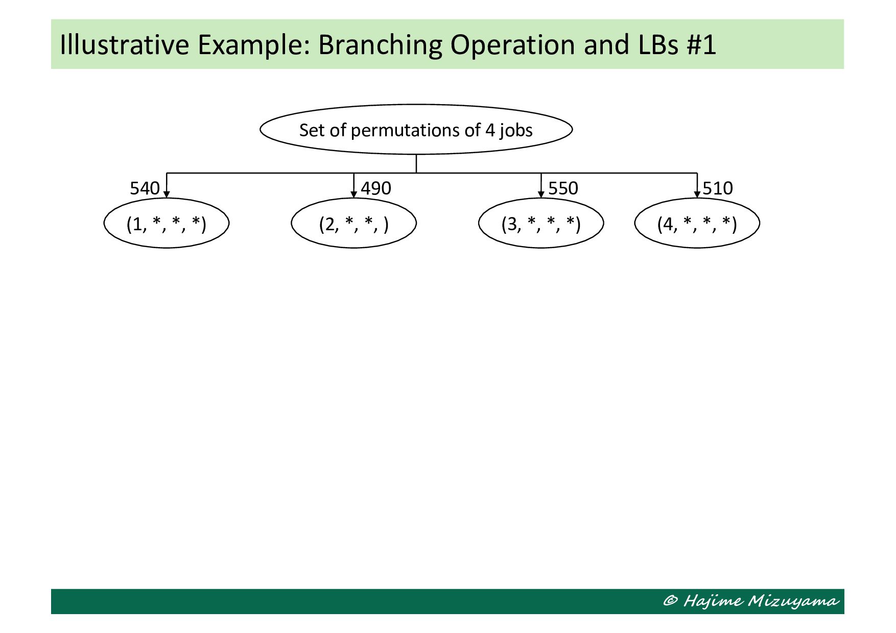
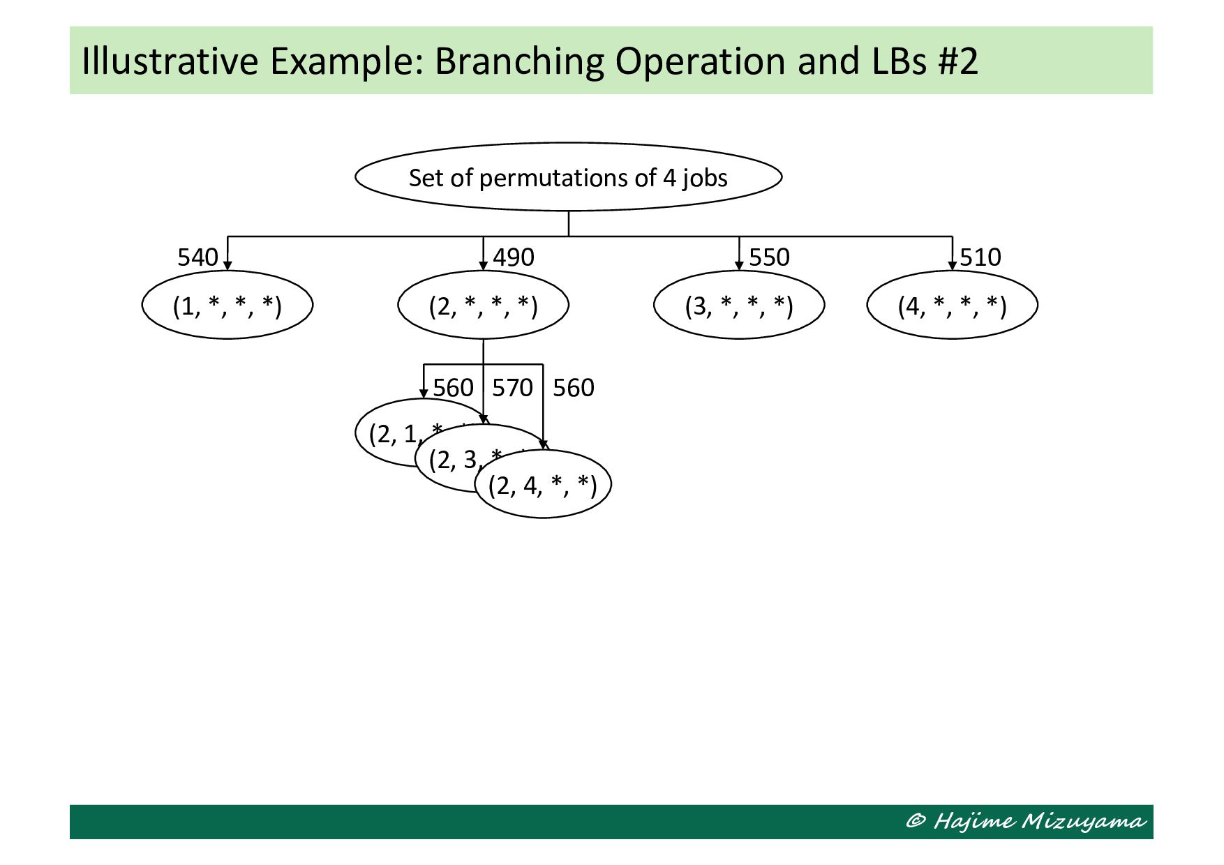
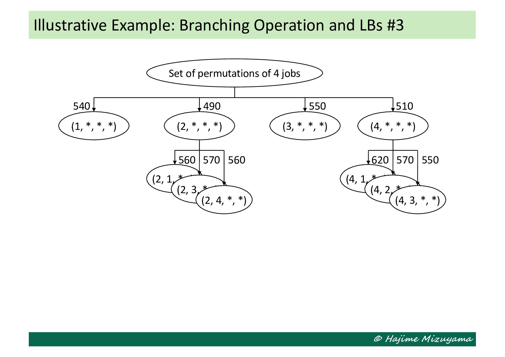
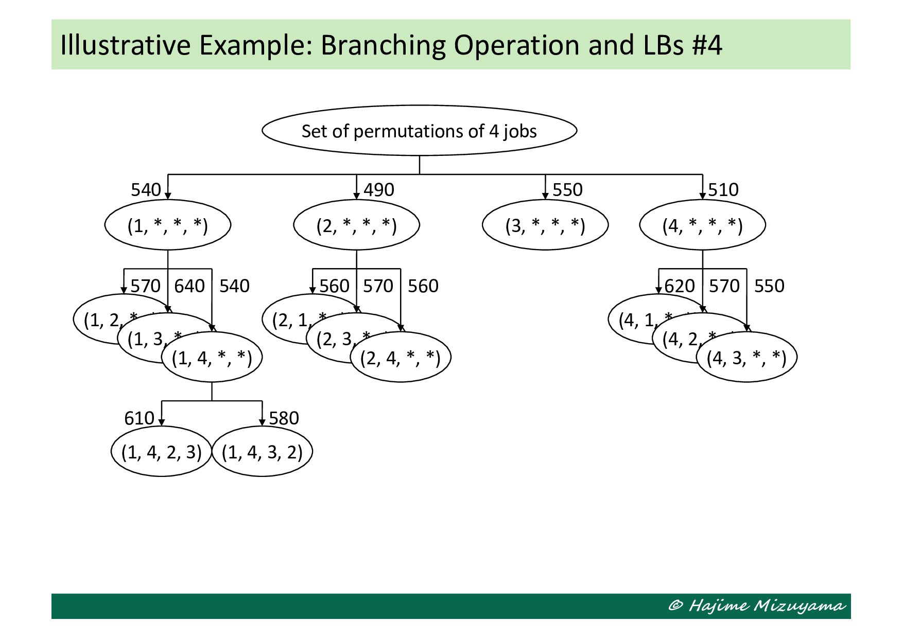
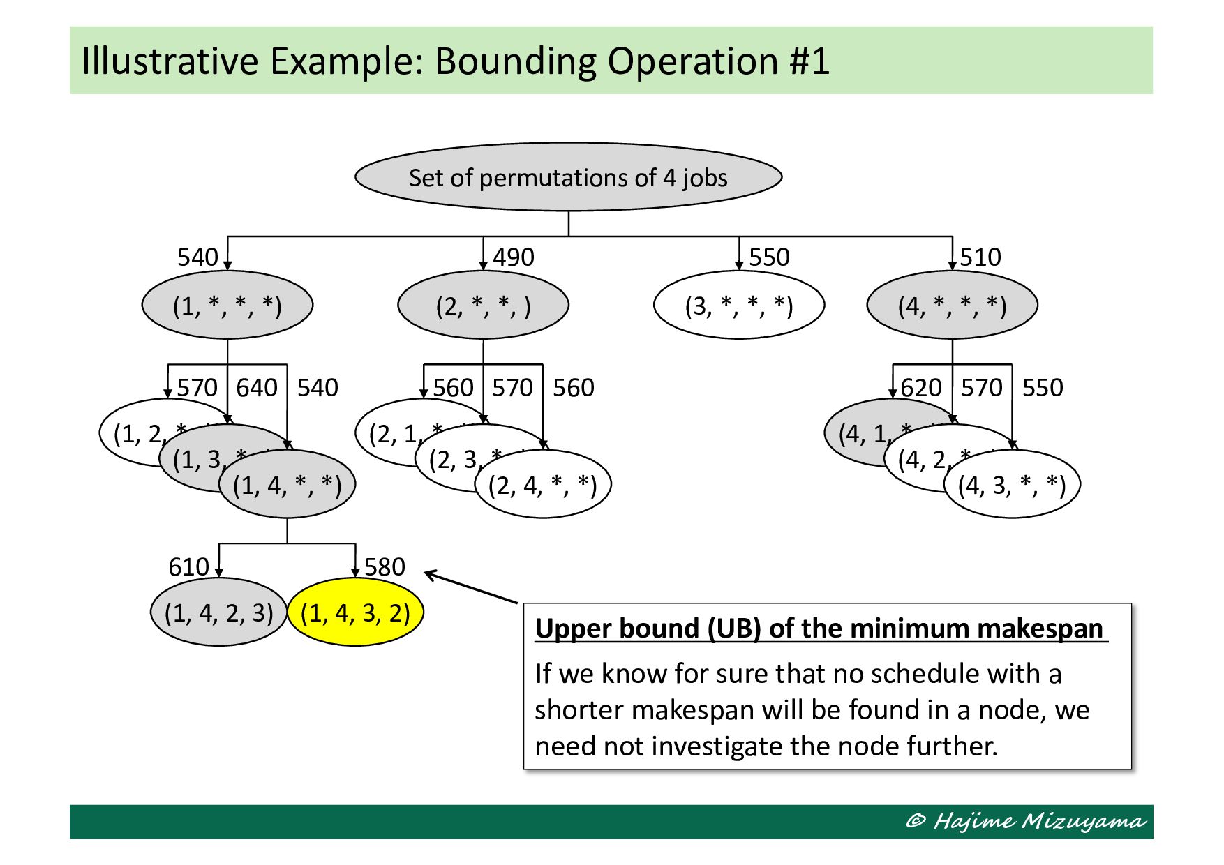
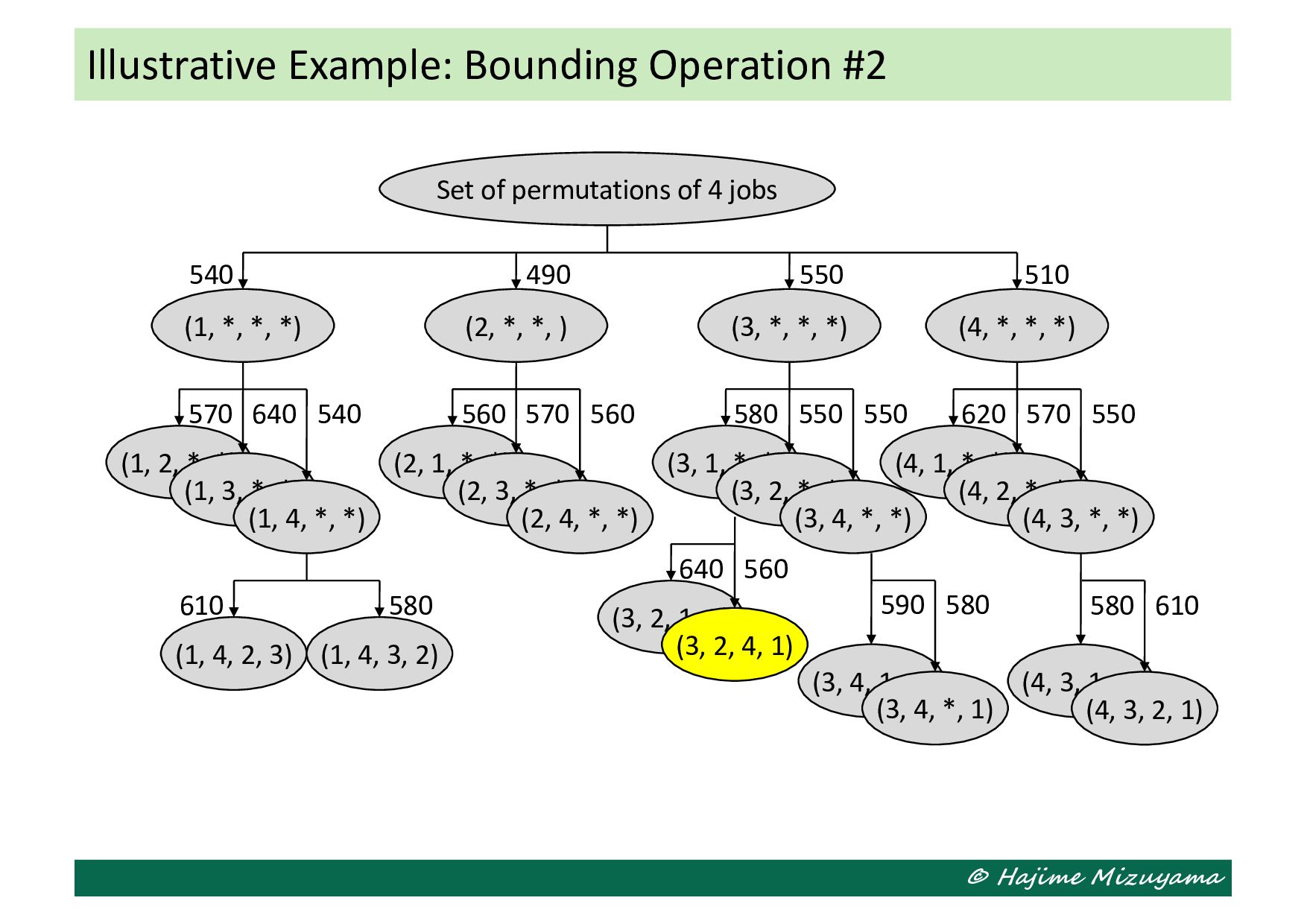
22. © Hajime Mizuyama 560 640 (4, 1, *, *) (4, 2, *, *) (2, 1, *, *) (2, 3, *, *) (1, 2, *, *) (1, 3, *, *) Illustrative Example: Bounding Operation #2 Set of permutations of 4 jobs (2, *, *, ) (1, *, *, *) (4, *, *, *) (3, *, *, *) (2, 4, *, *) 560 570 560 (4, 3, *, *) 570 550 (1, 4, *, *) 570 (1, 4, 2, 3) (1, 4, 3, 2) 580 (3, 1, *, *) (3, 2, *, *) (3, 4, *, *) 550 550 580 540 490 550 510 640 540 610 620 (4, 3, 1, 2) (4, 3, 2, 1) 580 610 (3, 4, 1, 2) (3, 4, *, 1) 590 580 (3, 2, 1, 2) (3, 2, 4, 1)
23. © Hajime Mizuyama Optimal Schedule in No Buffer Capacity Case M1 M2 M3 M4 J1 J2 J3 J4 𝑝!" 40 80 50 110 𝑝!# 120 30 80 50 𝑝!$ 90 60 130 20 𝑝!% 30 60 60 140 Processing times (min.) 𝐶&'( = 560 𝜋 = (3, 2, 4, 1)
24. © Hajime Mizuyama Precedence Diagram of Optimal Schedule (1, 1) (2, 1) (3, 1) (4, 1) (1, 2) (2, 2) (3, 2) (4, 2) (1, 3) (2, 3) (3, 3) (4, 3) (1, 4) (2, 4) (3, 4) (4, 4) Start End J3 J2 J4 J1 M1 M2 M3 M4 40 80 110 50 120 30 50 80 90 60 20 130 140 50 50 130 130 130 260 260 260 260 320 320 320 380 440 530 0 0 30 60 60 320 380 520 560 0
25. © Hajime Mizuyama Optimal Schedule in Unlimited Buffer Capacity Case J1 J2 J3 J4 𝑝!" 40 80 50 110 𝑝!# 120 30 80 50 𝑝!$ 90 60 130 20 𝑝!% 30 60 60 140 Processing times (min.) M1 M2 M3 M4 𝐶&'( = 540 𝜋 = (1, 4, 3, 2)
26. © Hajime Mizuyama Precedence Diagram of Optimal Schedule (1, 1) (4, 2) (3, 1) (2, 1) (1, 2) (4, 2) (3, 2) (2, 2) (1, 3) (4, 3) (3, 3) (2, 3) (1, 4) (4, 4) (3, 4) (2, 4) Start End J1 J4 J3 J2 M1 M2 M3 M4 0 40 40 110 80 50 120 50 30 80 90 20 60 130 110 50 120 50 80 90 20 130 30 140 60 60 0 40 160 250 40 160 250 280 150 210 290 420 200 290 420 480 540 0