Lecture slides for POM 2-14

生産管理技術2の講義14のスライドです．

Transcript

1. © Hajime Mizuyama Production & Operations Management #2 @AGU Lec.14: Supply Chain Management #2 • Double marginalization • Stackelberg game model • Newsvendor model
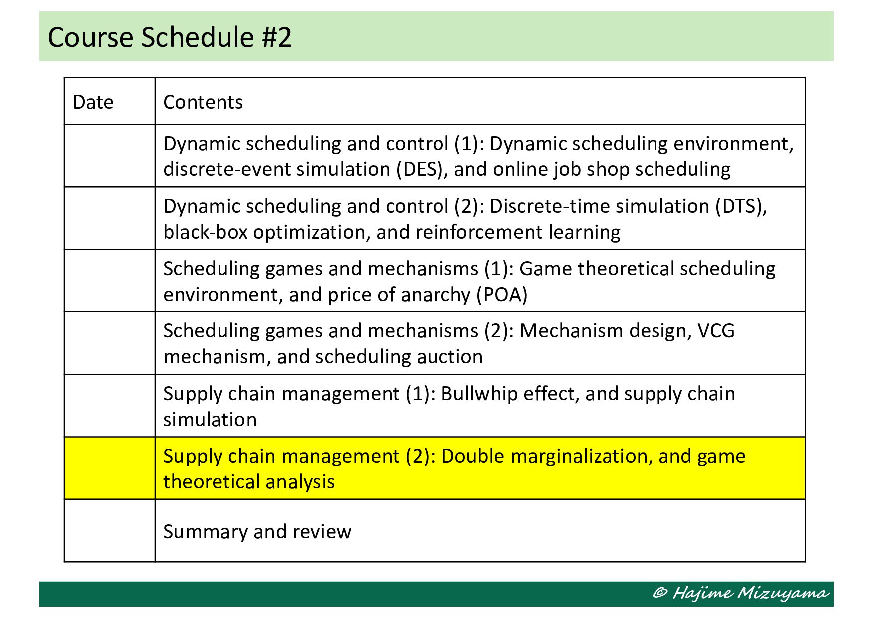
2. © Hajime Mizuyama Course Schedule #2 Date Contents Dynamic scheduling and control (1): Dynamic scheduling environment, discrete-event simulation (DES), and online job shop scheduling Dynamic scheduling and control (2): Discrete-time simulation (DTS), black-box optimization, and reinforcement learning Scheduling games and mechanisms (1): Game theoretical scheduling environment, and price of anarchy (POA) Scheduling games and mechanisms (2): Mechanism design, VCG mechanism, and scheduling auction Supply chain management (1): Bullwhip effect, and supply chain simulation Supply chain management (2): Double marginalization, and game theoretical analysis Summary and review
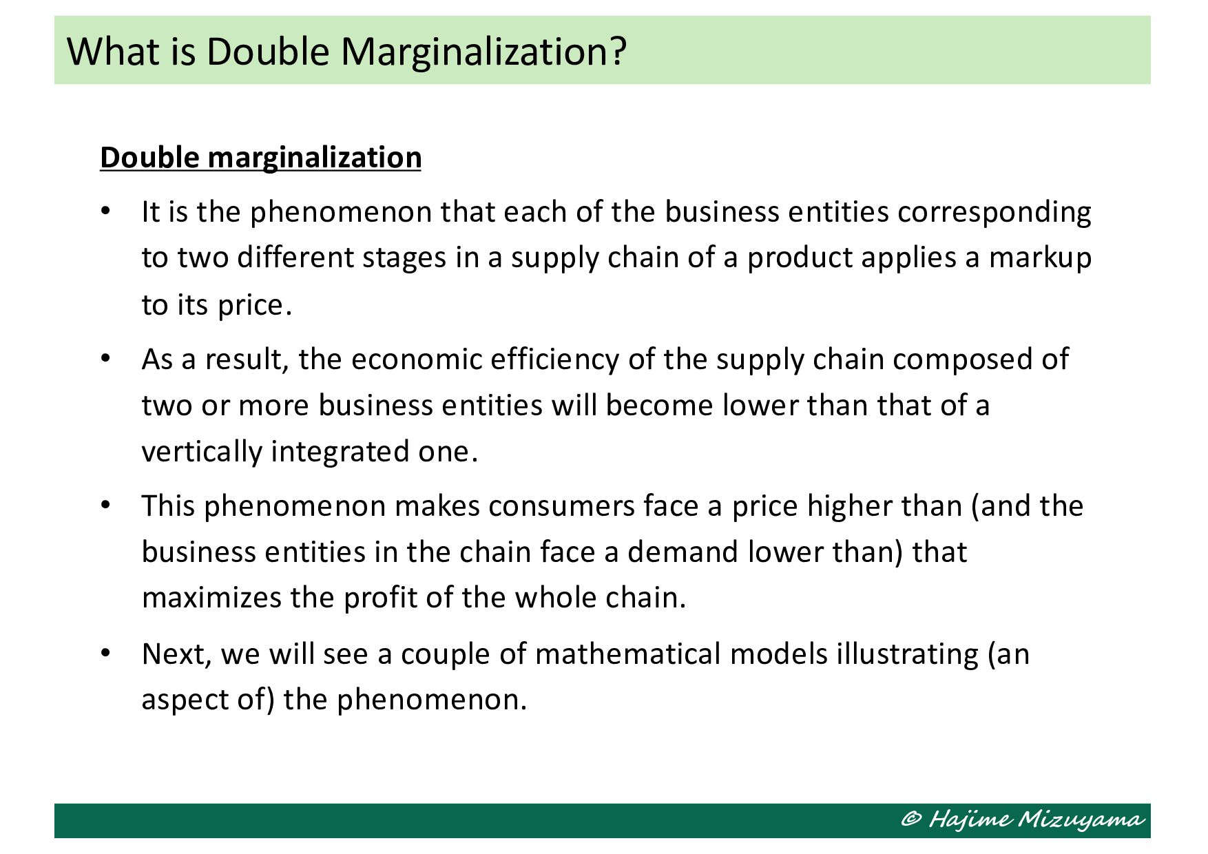
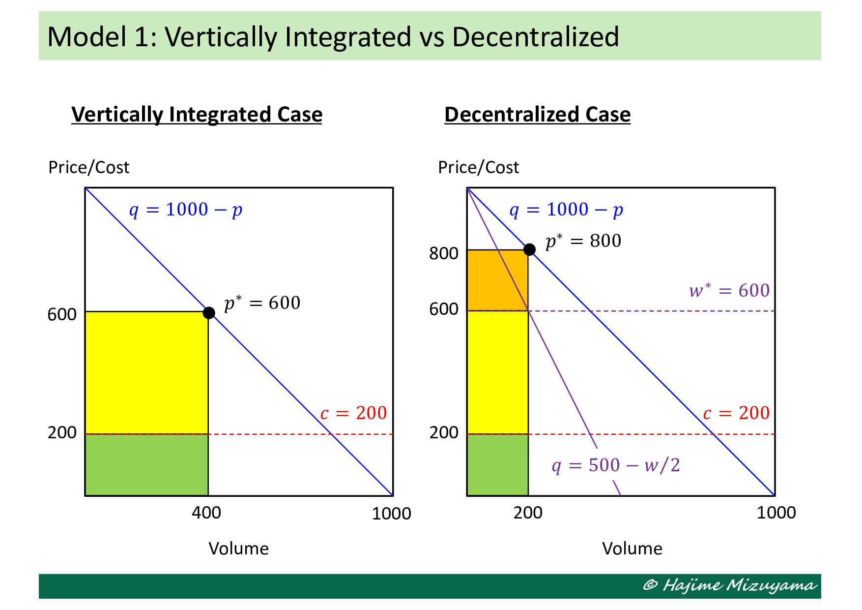
3. © Hajime Mizuyama Double marginalization • It is the phenomenon that each of the business entities corresponding to two different stages in a supply chain of a product applies a markup to its price. • As a result, the economic efficiency of the supply chain composed of two or more business entities will become lower than that of a vertically integrated one. • This phenomenon makes consumers face a price higher than (and the business entities in the chain face a demand lower than) that maximizes the profit of the whole chain. • Next, we will see a couple of mathematical models illustrating (an aspect of) the phenomenon. What is Double Marginalization?
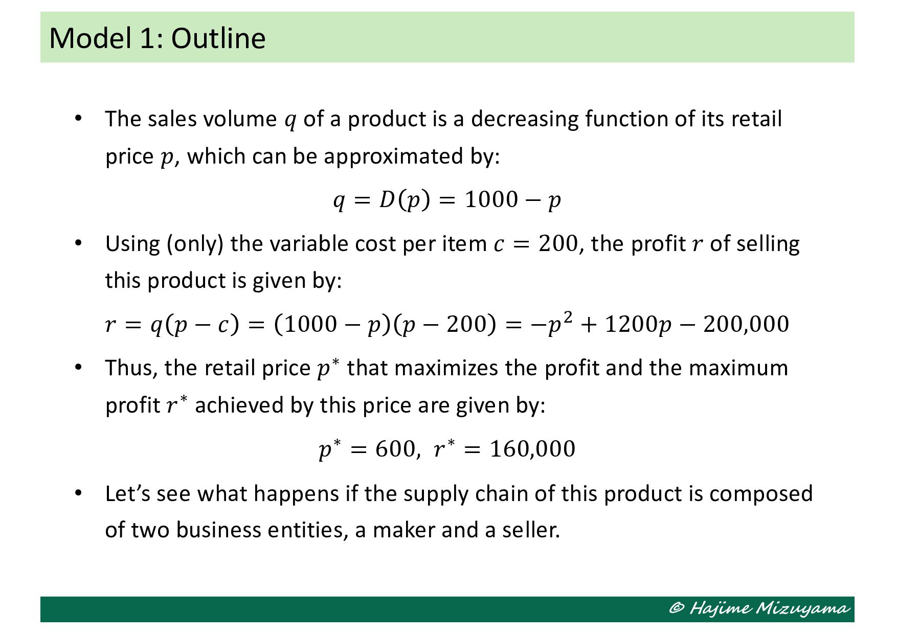
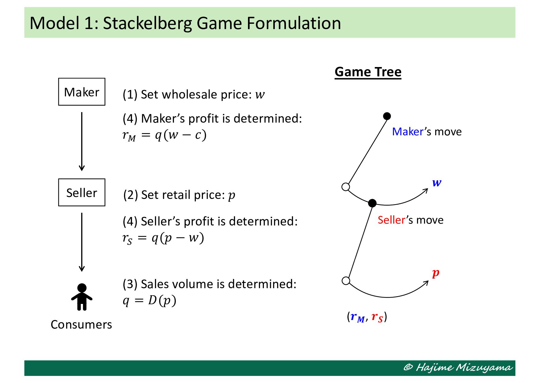
4. © Hajime Mizuyama • The sales volume 𝑞 of a product is a decreasing function of its retail price 𝑝, which can be approximated by: 𝑞 = 𝐷 𝑝 = 1000 − 𝑝 • Using (only) the variable cost per item 𝑐 = 200, the profit 𝑟 of selling this product is given by: 𝑟 = 𝑞 𝑝 − 𝑐 = 1000 − 𝑝 𝑝 − 200 = −𝑝! + 1200𝑝 − 200,000 • Thus, the retail price 𝑝∗ that maximizes the profit and the maximum profit 𝑟∗ achieved by this price are given by: 𝑝∗ = 600, 𝑟∗ = 160,000 • Let’s see what happens if the supply chain of this product is composed of two business entities, a maker and a seller. Model 1: Outline
5. © Hajime Mizuyama Model 1: Stackelberg Game Formulation Maker Seller Consumers (1) Set wholesale price: 𝑤 (2) Set retail price: 𝑝 (3) Sales volume is determined: 𝑞 = 𝐷(𝑝) (4) Seller’s profit is determined: 𝑟! = 𝑞(𝑝 − 𝑤) (4) Maker’s profit is determined: 𝑟" = 𝑞(𝑤 − 𝑐) Maker’s move Seller’s move (𝒓𝑴, 𝒓𝑺) Game Tree 𝒘 𝒑
6. © Hajime Mizuyama Seller’s Decision • To maximize the profit 𝑟# = 1000 − 𝑝 𝑝 − 𝑤 , the retail price should be set as 𝑝∗ = ⁄ (1000 + 𝑤) 2 = 500 + 𝑤/2. Maker’s Decision • To maximize the profit 𝑟$ = 1000 − 𝑝∗ 𝑤 − 200 = (1000 − 𝑤)(𝑤 − 200)/2, the wholesale price should be set as: 𝑤∗ = 600. Result • Since 𝑤∗ = 600, we have 𝑝∗ = 800, and 𝑞 = 1000 − 800 = 200. • Thus, profits are 𝑟$ ∗ = 80,000, and 𝑟# ∗ = 40,000. • So unfortunately, 𝑟$ ∗ + 𝑟# ∗ = 120,000 < 160,000 = 𝑟∗. Model 1: Decisions of Players (Equilibrium)
7. © Hajime Mizuyama Model 1: Vertically Integrated vs Decentralized Vertically Integrated Case Decentralized Case Volume Volume Price/Cost Price/Cost 600 200 𝑞 = 1000 − 𝑝 400 𝑐 = 200 𝑞 = 1000 − 𝑝 𝑐 = 200 200 600 800 𝑝∗ = 600 𝑝∗ = 800 𝑤∗ = 600 200 𝑞 = 500 − ⁄ 𝑤 2 1000 1000
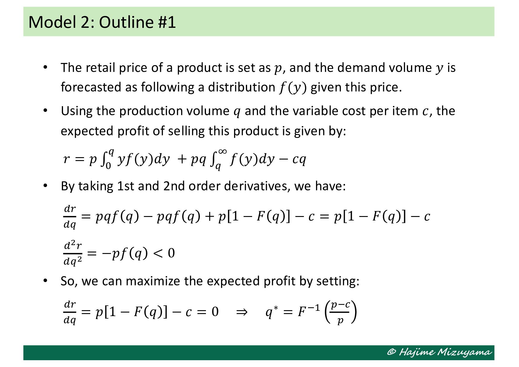
8. © Hajime Mizuyama • The retail price of a product is set as 𝑝, and the demand volume 𝑦 is forecasted as following a distribution 𝑓(𝑦) given this price. • Using the production volume 𝑞 and the variable cost per item 𝑐, the expected profit of selling this product is given by: 𝑟 = 𝑝 ∫ % & 𝑦𝑓(𝑦)𝑑𝑦 + 𝑝𝑞 ∫ & ' 𝑓(𝑦)𝑑𝑦 − 𝑐𝑞 • By taking 1st and 2nd order derivatives, we have: () (& = 𝑝𝑞𝑓 𝑞 − 𝑝𝑞𝑓 𝑞 + 𝑝 1 − 𝐹 𝑞 − 𝑐 = 𝑝 1 − 𝐹 𝑞 − 𝑐 ($) (&$ = −𝑝𝑓 𝑞 < 0 • So, we can maximize the expected profit by setting: () (& = 𝑝 1 − 𝐹 𝑞 − 𝑐 = 0 ⇒ 𝑞∗ = 𝐹*+ ,*- , Model 2: Outline #1
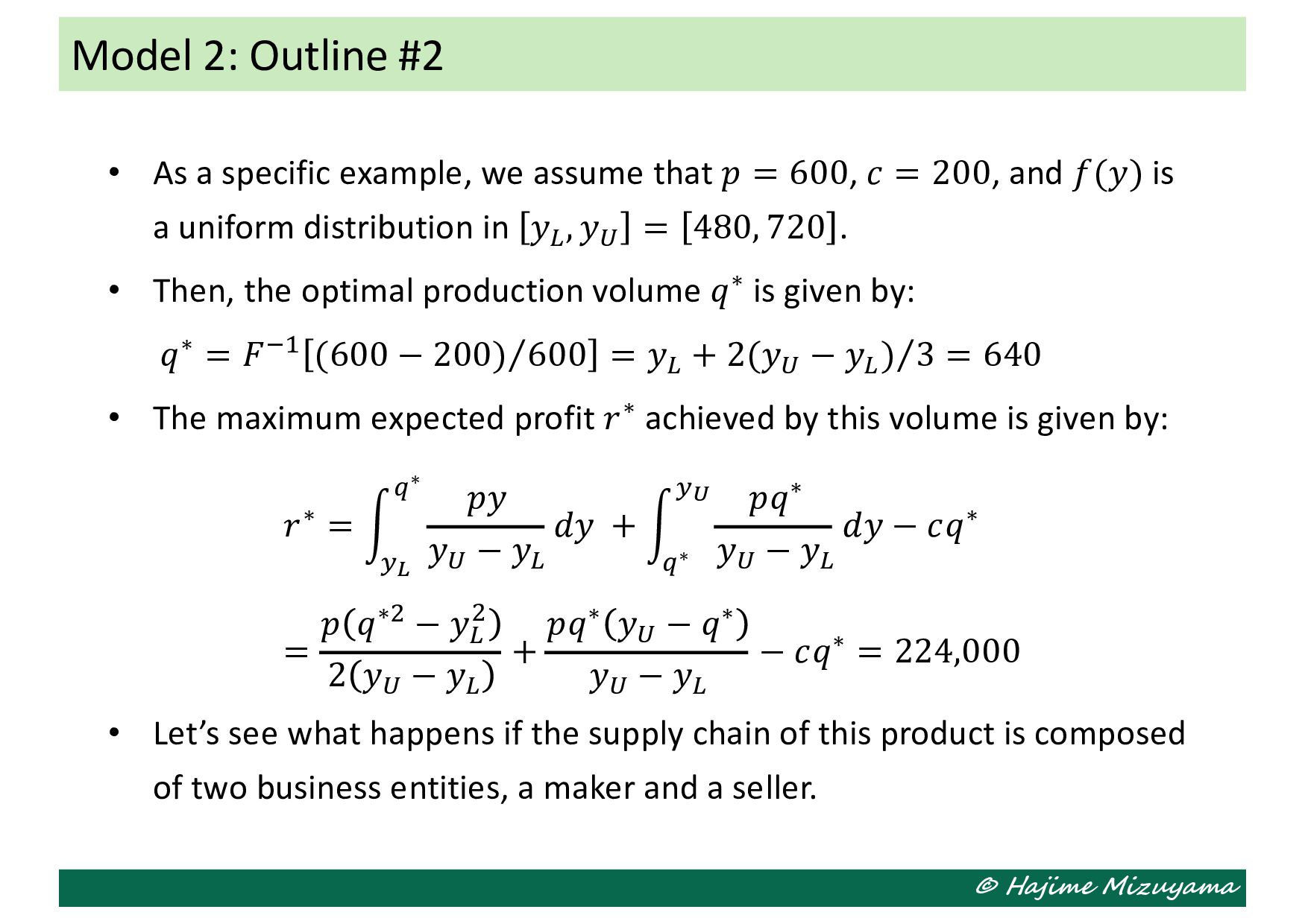
9. © Hajime Mizuyama • As a specific example, we assume that 𝑝 = 600, 𝑐 = 200, and 𝑓(𝑦) is a uniform distribution in 𝑦. , 𝑦/ = 480, 720 . • Then, the optimal production volume 𝑞∗ is given by: 𝑞∗ = 𝐹*+ ⁄ (600 − 200) 600 = 𝑦. + ⁄ 2(𝑦/ − 𝑦. ) 3 = 640 • The maximum expected profit 𝑟∗ achieved by this volume is given by: 𝑟∗ = ? 0% &∗ 𝑝𝑦 𝑦/ − 𝑦. 𝑑𝑦 + ? &∗ 0& 𝑝𝑞∗ 𝑦/ − 𝑦. 𝑑𝑦 − 𝑐𝑞∗ = 𝑝 𝑞∗! − 𝑦. ! 2 𝑦/ − 𝑦. + 𝑝𝑞∗ 𝑦/ − 𝑞∗ 𝑦/ − 𝑦. − 𝑐𝑞∗ = 224,000 • Let’s see what happens if the supply chain of this product is composed of two business entities, a maker and a seller. Model 2: Outline #2
10. © Hajime Mizuyama • Suppose that the maker has set the wholesale price as 𝑤 = 400. • Then, the expected profit of the seller is given by: 𝑟# = 𝑝 ∫ % & 𝑦𝑓(𝑦)𝑑𝑦 + 𝑝𝑞 ∫ & ' 𝑓(𝑦)𝑑𝑦 − 𝑤𝑞 • Thus, the purchase volume 𝑞∗ that maximizes the expected profit and the maximum expected profit 𝑟# ∗ achieved by this volume are: 𝑞∗ = 𝐹*+ ⁄ 𝑝 − 𝑤 𝑝 = 𝑦. + ⁄ (𝑦/ − 𝑦. ) 3 = 560 𝑟# ∗ = , &∗$*0% $ !(0&*0%) + ,&∗(0&*&∗) 0&*0% − 𝑤𝑞∗ = 104,000 • As a result, the profit of the maker and the total expected profit are: 𝑟$ = 𝑤 − 𝑐 𝑞∗ = (400 − 200)×560 = 112,000 𝑟$ + 𝑟# ∗ = 112,000 + 104,000 = 216,000 < 224,000 = 𝑟∗ Model 2: Newsvendor Formulation
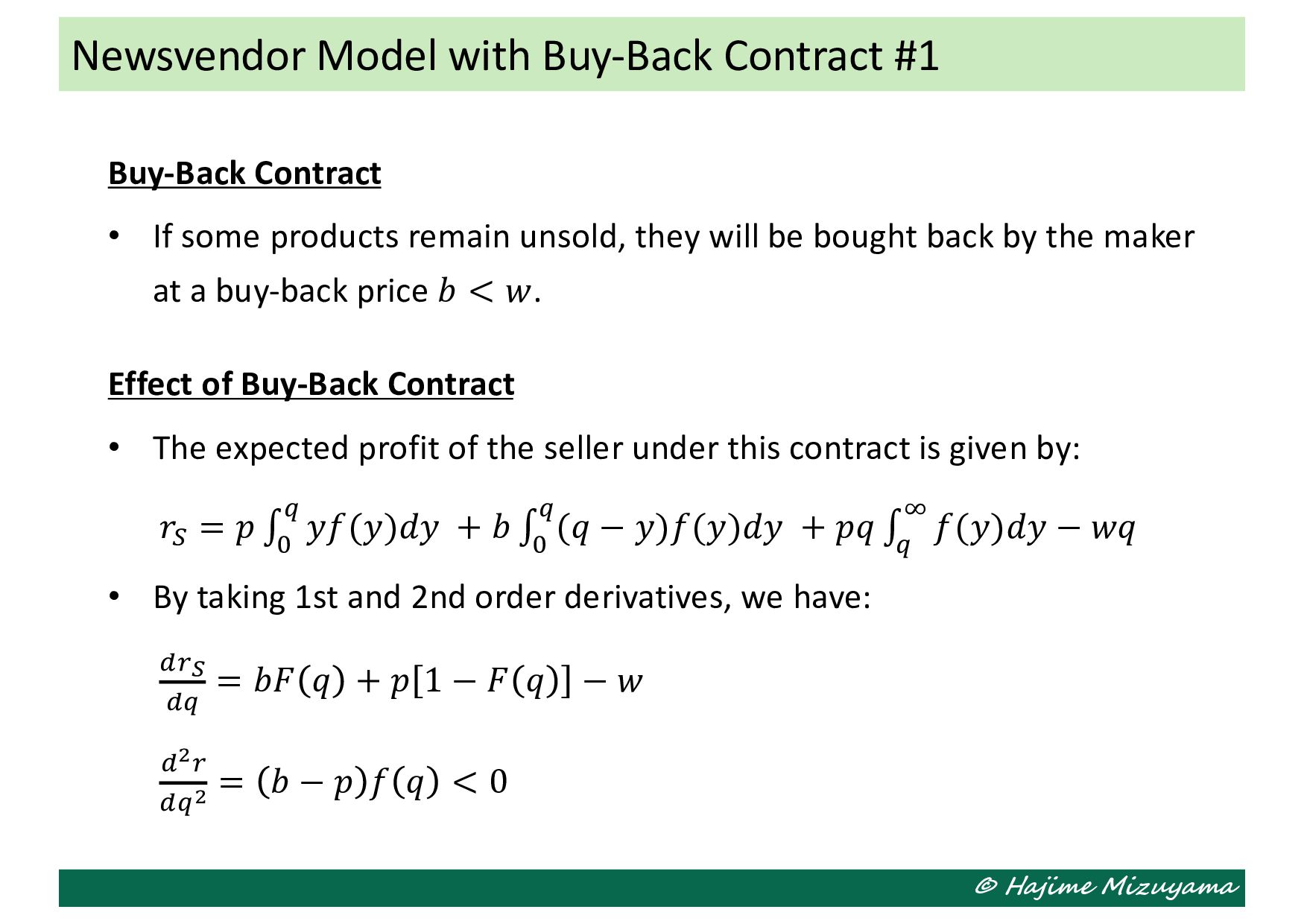
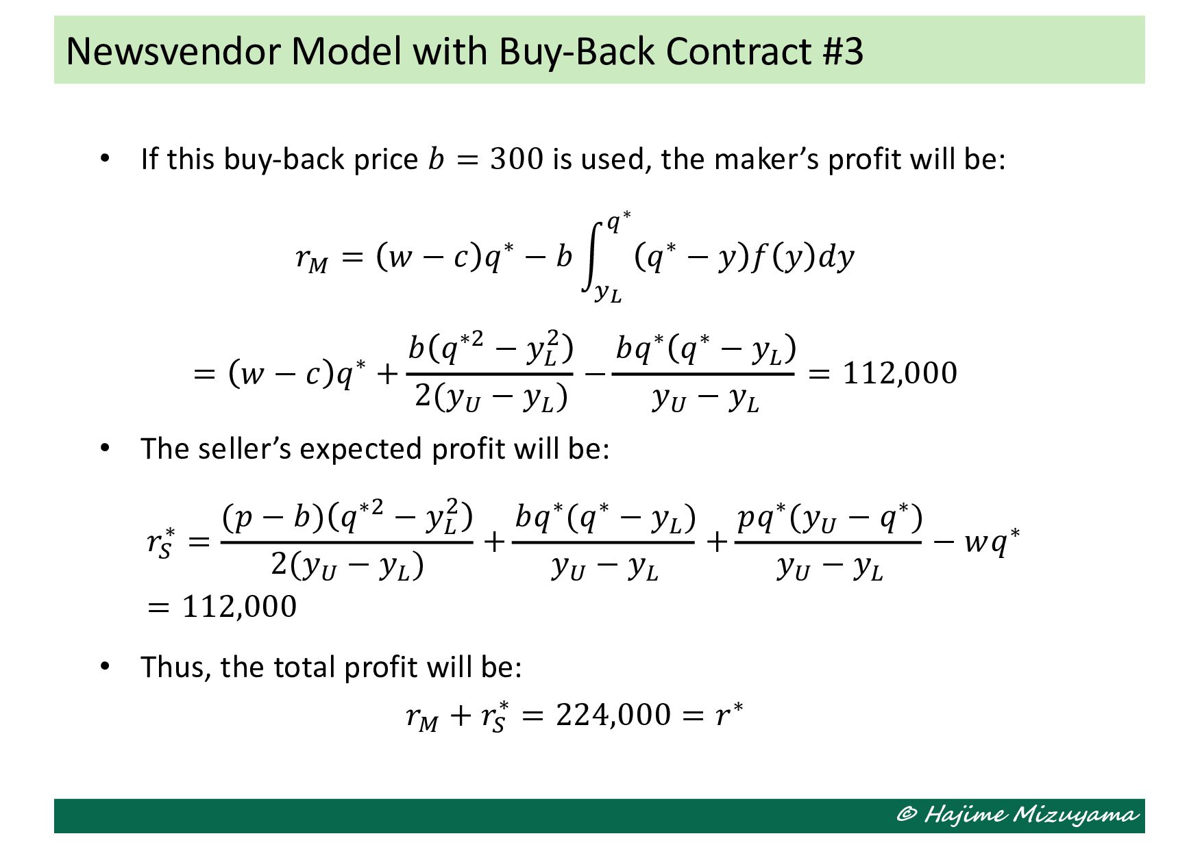
11. © Hajime Mizuyama Buy-Back Contract • If some products remain unsold, they will be bought back by the maker at a buy-back price 𝑏 < 𝑤. Effect of Buy-Back Contract • The expected profit of the seller under this contract is given by: 𝑟# = 𝑝 ∫ % & 𝑦𝑓(𝑦)𝑑𝑦 + 𝑏 ∫ % & (𝑞 − 𝑦)𝑓(𝑦)𝑑𝑦 + 𝑝𝑞 ∫ & ' 𝑓(𝑦)𝑑𝑦 − 𝑤𝑞 • By taking 1st and 2nd order derivatives, we have: ()' (& = 𝑏𝐹 𝑞 + 𝑝 1 − 𝐹 𝑞 − 𝑤 ($) (&$ = 𝑏 − 𝑝 𝑓 𝑞 < 0 Newsvendor Model with Buy-Back Contract #1
12. © Hajime Mizuyama • So, the seller can maximize its expected profit by setting: 𝑑𝑟# 𝑑𝑞 = 𝑏𝐹 𝑞 + 𝑝 1 − 𝐹 𝑞 − 𝑤 = 0 ⇒ 𝑞∗ = 𝐹*+ 𝑝 − 𝑤 𝑝 − 𝑏 • Thus, with this contract, the decentralized supply chain may be made as efficient as the vertically integrated one (𝑞∗ = 640) by setting: (𝑝 − 𝑤) 𝑝 − 𝑏 = (𝑝 − 𝑐) 𝑝 ⇒ 𝑏 = 𝑝(𝑤 − 𝑐) (𝑝 − 𝑐) = 600 400 − 200 600 − 200 = 300 Newsvendor Model with Buy-Back Contract #2
13. © Hajime Mizuyama • If this buy-back price 𝑏 = 300 is used, the maker’s profit will be: 𝑟$ = 𝑤 − 𝑐 𝑞∗ − 𝑏 ? 0% &∗ 𝑞∗ − 𝑦 𝑓 𝑦 𝑑𝑦 = 𝑤 − 𝑐 𝑞∗ + 𝑏 𝑞∗! − 𝑦. ! 2(𝑦/ − 𝑦. ) − 𝑏𝑞∗ 𝑞∗ − 𝑦. 𝑦/ − 𝑦. = 112,000 • The seller’s expected profit will be: 𝑟# ∗ = (𝑝 − 𝑏) 𝑞∗! − 𝑦. ! 2(𝑦/ − 𝑦. ) + 𝑏𝑞∗(𝑞∗ − 𝑦. ) 𝑦/ − 𝑦. + 𝑝𝑞∗(𝑦/ − 𝑞∗) 𝑦/ − 𝑦. − 𝑤𝑞∗ = 112,000 • Thus, the total profit will be: 𝑟$ + 𝑟# ∗ = 224,000 = 𝑟∗ Newsvendor Model with Buy-Back Contract #3