Lecture slides for POM 2-5

生産管理技術2の講義5のスライドです．

Transcript

1. © Hajime Mizuyama Production & Operations Management #2 @AGU Lec.5: Metaheuristics • Global and local Optima • Neighborhood operations and naïve local search • Simulated annealing, tabu search, and genetic algorithm
2. © Hajime Mizuyama Course Schedule #2 Date Contents Single machine scheduling (1): Dynamic programming (DP) Single machine scheduling (2): Branch and bound (BAB) Flow shop scheduling: Unlimited, limited, and no buffer capacity cases, and branch and bound (BAB) Metaheuristics: Local search, simulated annealing, tabu search, genetic algorithm, etc. Job shop scheduling (1): Disjunctive graph representation, and 0-1 mixed-integer linear programming (0-1 MILP) formulation Job shop scheduling (2): How to enumerate active schedules, and branch and bound (BAB) Mid-term examination
3. © Hajime Mizuyama • Solution space (i.e., the set of feasible schedules): Π For example, in the single machine and flow shop scheduling problems addressed so far, this is the set of job permutations. • Objective function (to be minimized) of a schedule 𝜋 ∈ Π: 𝑓(𝜋) • Neighborhood of a schedule 𝜋 ∈ Π: 𝑁(𝜋) This is a set of schedules that are similar, in a specified sense, to 𝜋. • Global optimum: 𝜋∗ ∈ argmin "∈$ 𝑓(𝜋) • Local optimum: 𝜋⋆ ∈ 𝜋 𝑓 𝜋 ≤ 𝑓 𝜋& ∀ 𝜋& ∈ 𝑁 𝜋 } Every global optimum is also locally optimal, but a local optimum is not necessarily globally optimal. Global and Local Optimum
4. © Hajime Mizuyama Choose an initial schedule 𝜋' ∈ Π at random or according to a heuristic. 𝜋⋆ ← 𝜋'; 𝑓⋆ ← 𝑓(𝜋' ); 2 Π ← 𝑁(𝜋' ); 𝑖 ← 1 while 2 Π ≠ ∅ do Choose a schedule 𝜋 ∈ 2 Π at random. 2 Π ← 2 Π ∖ 𝜋 Evaluate 𝑓 𝜋 . if 𝑓 𝜋 < 𝑓⋆ then (that is, if 𝜋 is strictly better than 𝜋⋆) 𝜋⋆ ← 𝜋; 𝑓⋆ ← 𝑓(𝜋); 2 Π ← 𝑁(𝜋) 𝜋( ← 𝜋; 𝑖 ← 𝑖 + 1 fi od Algorithm of Naïve Local Search
5. © Hajime Mizuyama Schema of Local Search 𝜋! 𝑁(𝜋! ) Local optimum No better schedule is found in the neighborhood. 𝜋" 𝜋# 𝜋$ 𝜋% 𝜋& 𝜋'
6. © Hajime Mizuyama • Adjacent pairwise interchange operator • Exchange operator • Insertion operator Typical Neighborhood Operators for Job Permutation 1st 2nd 3rd 𝑘 th 𝑘 + 1 th |𝐽| th 1st 2nd 3rd 𝑘 th 𝑙 th |𝐽| th 1st 2nd 3rd 𝑘 th |𝐽| th … … … … … … … … exchange exchange insert
7. © Hajime Mizuyama Illustrative Example Flow shop scheduling problem to minimize makespan with no buffer capacity between machines Let us follow the process of naïve local search in adjacent pairwise interchange neighborhood from initial solution 𝜋' = (1, 2, 3, 4). M1 M2 M3 M4 J1 J2 J3 J4 𝑝!" 40 80 50 110 𝑝!# 120 30 80 50 𝑝!$ 90 60 130 20 𝑝!% 30 60 60 140 Processing times (min.) 𝐶/01 = 660 Blocking
8. © Hajime Mizuyama 𝜋 𝐶&'( Solution trajectory 𝜋 𝐶&'( Solution trajectory (1, 2, 3, 4) 660 𝜋) (3, 1, 2, 4) (1, 2, 4, 3) (3, 1, 4, 2) (1, 3, 2, 4) (3, 2, 1, 4) (1, 3, 4, 2) (3, 2, 4, 1) (1, 4, 2, 3) (3, 4, 1, 2) (1, 4, 3, 2) (3, 4, 2, 1) (2, 1, 3, 4) (4, 1, 2, 3) (2, 1, 4, 3) (4, 1, 3, 2) (2, 3, 1, 4) (4, 2, 1, 3) (2, 3, 4, 1) (4, 2, 3, 1) (2, 4, 1, 3) (4, 3, 1, 2) (2, 4, 3, 1) (4, 3, 2, 1) illustrative Example: Iteration 0
9. © Hajime Mizuyama 𝜋 𝐶&'( Solution trajectory 𝜋 𝐶&'( Solution trajectory (1, 2, 3, 4) 660 𝜋) (3, 1, 2, 4) (1, 2, 4, 3) 590 (3, 1, 4, 2) (1, 3, 2, 4) 640 𝜋" (3, 2, 1, 4) (1, 3, 4, 2) (3, 2, 4, 1) (1, 4, 2, 3) (3, 4, 1, 2) (1, 4, 3, 2) (3, 4, 2, 1) (2, 1, 3, 4) 660 (4, 1, 2, 3) (2, 1, 4, 3) (4, 1, 3, 2) (2, 3, 1, 4) (4, 2, 1, 3) (2, 3, 4, 1) (4, 2, 3, 1) (2, 4, 1, 3) (4, 3, 1, 2) (2, 4, 3, 1) (4, 3, 2, 1) illustrative Example: Iteration 1
10. © Hajime Mizuyama 𝜋 𝐶&'( Solution trajectory 𝜋 𝐶&'( Solution trajectory (1, 2, 3, 4) 660 𝜋) (3, 1, 2, 4) 610 𝜋# (1, 2, 4, 3) (3, 1, 4, 2) (1, 3, 2, 4) 640 𝜋" (3, 2, 1, 4) (1, 3, 4, 2) 640 (3, 2, 4, 1) (1, 4, 2, 3) (3, 4, 1, 2) (1, 4, 3, 2) (3, 4, 2, 1) (2, 1, 3, 4) (4, 1, 2, 3) (2, 1, 4, 3) (4, 1, 3, 2) (2, 3, 1, 4) (4, 2, 1, 3) (2, 3, 4, 1) (4, 2, 3, 1) (2, 4, 1, 3) (4, 3, 1, 2) (2, 4, 3, 1) (4, 3, 2, 1) illustrative Example: Iteration 2
11. © Hajime Mizuyama 𝜋 𝐶&'( Solution trajectory 𝜋 𝐶&'( Solution trajectory (1, 2, 3, 4) 660 𝜋) (3, 1, 2, 4) 610 𝜋# (1, 2, 4, 3) (3, 1, 4, 2) 580 𝜋$ (1, 3, 2, 4) 640 𝜋" (3, 2, 1, 4) 640 (1, 3, 4, 2) (3, 2, 4, 1) (1, 4, 2, 3) (3, 4, 1, 2) (1, 4, 3, 2) (3, 4, 2, 1) (2, 1, 3, 4) (4, 1, 2, 3) (2, 1, 4, 3) (4, 1, 3, 2) (2, 3, 1, 4) (4, 2, 1, 3) (2, 3, 4, 1) (4, 2, 3, 1) (2, 4, 1, 3) (4, 3, 1, 2) (2, 4, 3, 1) (4, 3, 2, 1) illustrative Example: Iteration 3
12. © Hajime Mizuyama 𝜋 𝐶&'( Solution trajectory 𝜋 𝐶&'( Solution trajectory (1, 2, 3, 4) 660 𝜋) (3, 1, 2, 4) 610 𝜋# (1, 2, 4, 3) (3, 1, 4, 2) 580 𝜋$ (1, 3, 2, 4) 640 𝜋" (3, 2, 1, 4) (1, 3, 4, 2) 640 (3, 2, 4, 1) (1, 4, 2, 3) (3, 4, 1, 2) 590 (1, 4, 3, 2) (3, 4, 2, 1) (2, 1, 3, 4) (4, 1, 2, 3) (2, 1, 4, 3) (4, 1, 3, 2) (2, 3, 1, 4) (4, 2, 1, 3) (2, 3, 4, 1) (4, 2, 3, 1) (2, 4, 1, 3) (4, 3, 1, 2) (2, 4, 3, 1) (4, 3, 2, 1) illustrative Example: Iteration 4
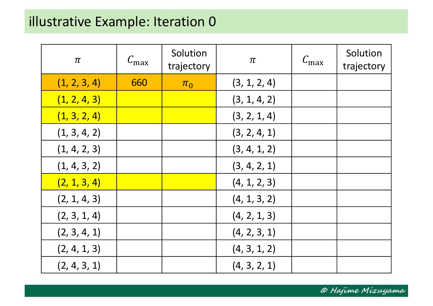
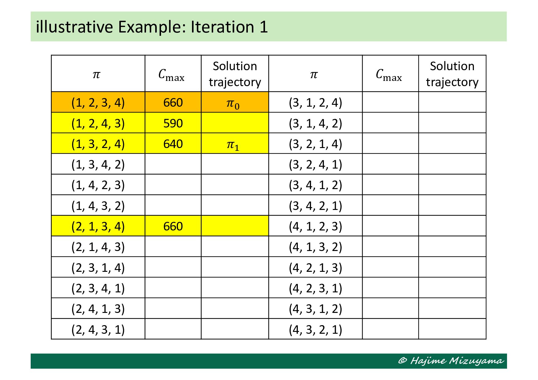
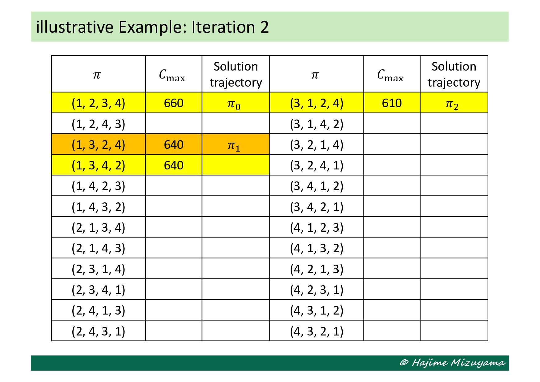
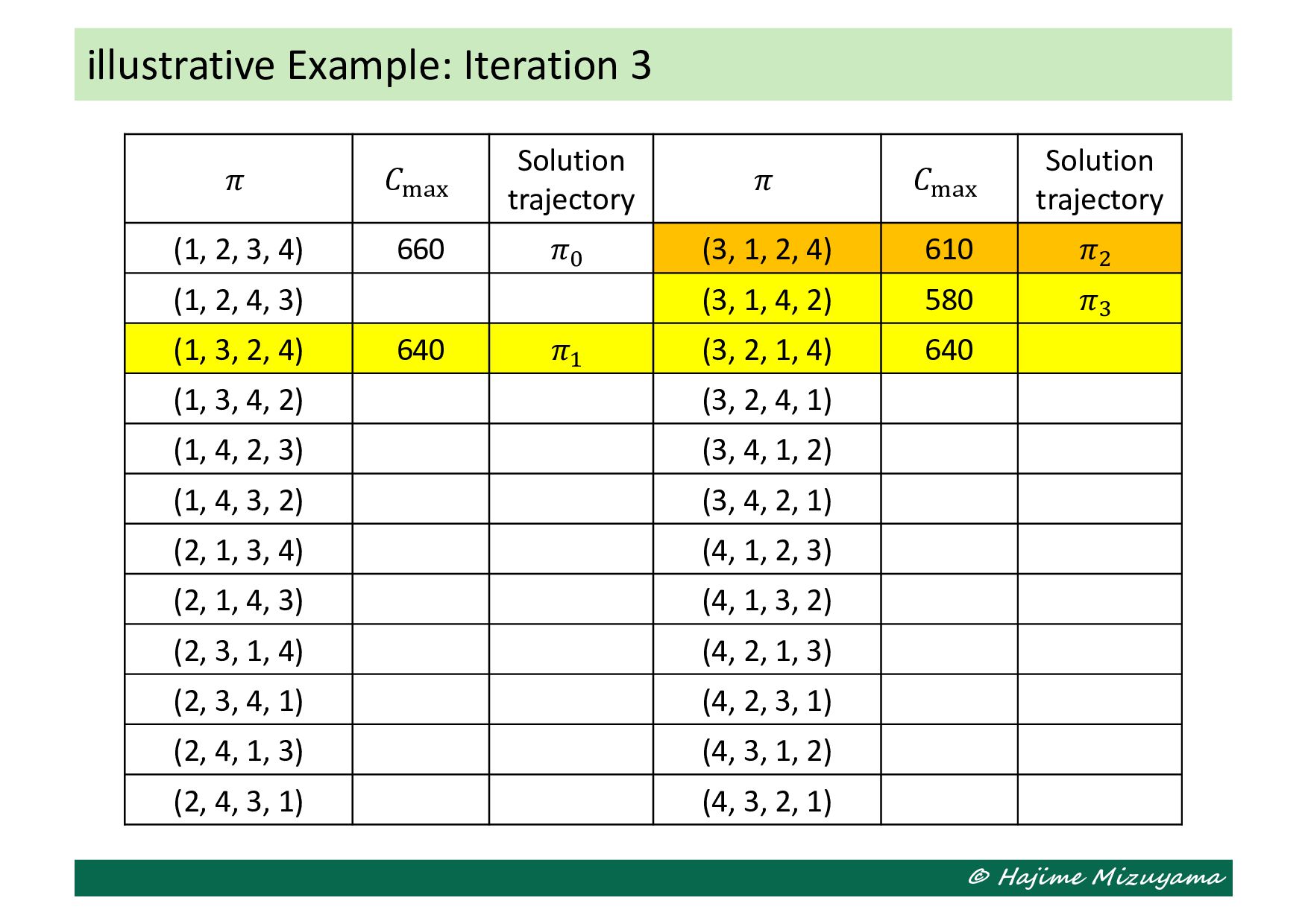
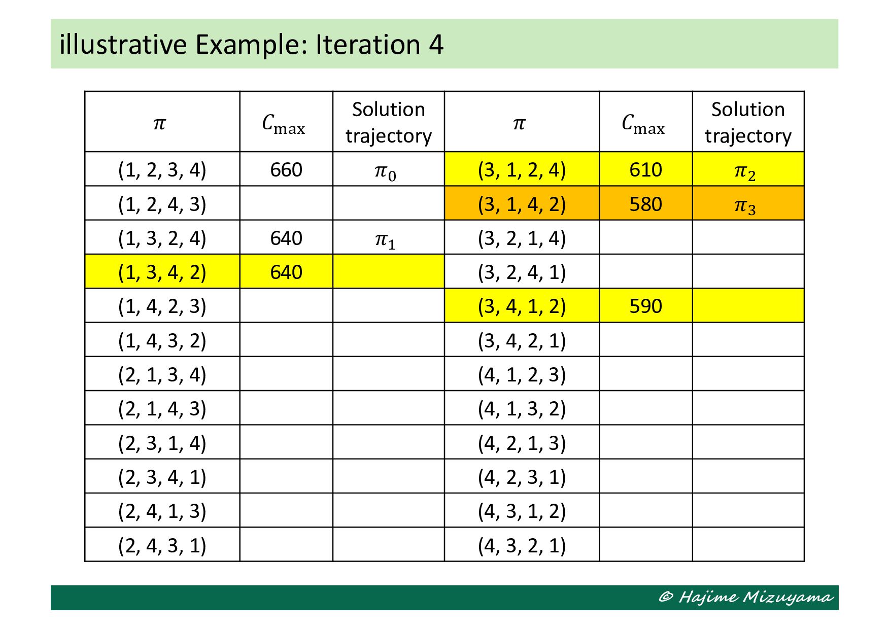
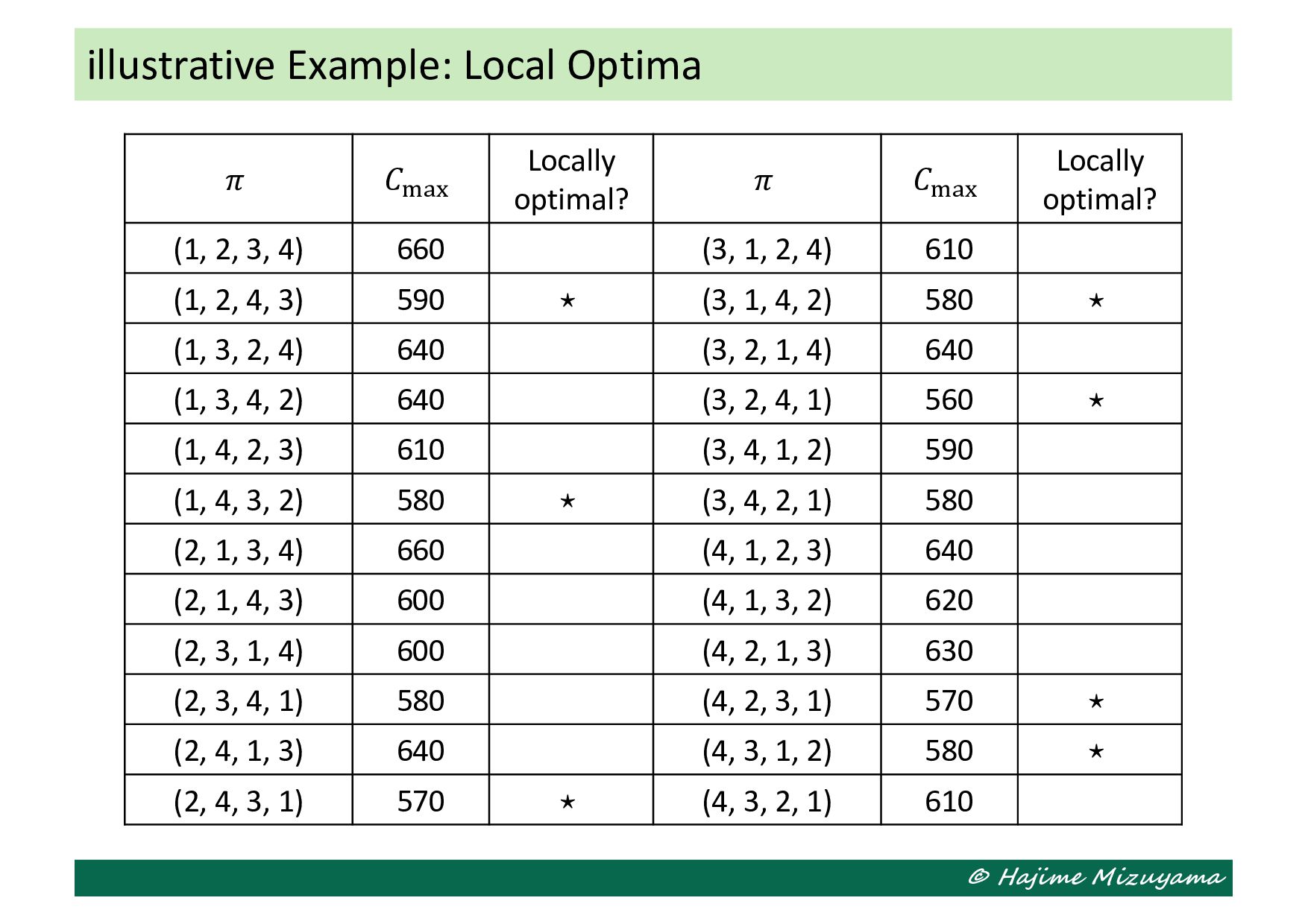
13. © Hajime Mizuyama 𝜋 𝐶&'( Locally optimal? 𝜋 𝐶&'( Locally optimal? (1, 2, 3, 4) 660 (3, 1, 2, 4) 610 (1, 2, 4, 3) 590 ⋆ (3, 1, 4, 2) 580 ⋆ (1, 3, 2, 4) 640 (3, 2, 1, 4) 640 (1, 3, 4, 2) 640 (3, 2, 4, 1) 560 ⋆ (1, 4, 2, 3) 610 (3, 4, 1, 2) 590 (1, 4, 3, 2) 580 ⋆ (3, 4, 2, 1) 580 (2, 1, 3, 4) 660 (4, 1, 2, 3) 640 (2, 1, 4, 3) 600 (4, 1, 3, 2) 620 (2, 3, 1, 4) 600 (4, 2, 1, 3) 630 (2, 3, 4, 1) 580 (4, 2, 3, 1) 570 ⋆ (2, 4, 1, 3) 640 (4, 3, 1, 2) 580 ⋆ (2, 4, 3, 1) 570 ⋆ (4, 3, 2, 1) 610 illustrative Example: Local Optima
14. © Hajime Mizuyama • The solution space of a scheduling problem may have many local optima, other than the globally optimal solutions. • The performance of such locally optimal solutions may not always be favorable but can be quite disappointing. • The naïve local search procedure stops at a local optimum, which, in many cases, is not globally optimal. • Accordingly, the local optimum found by the procedure may not necessarily be a satisfactory schedule. Limitations of Naïve Local Search
15. © Hajime Mizuyama • One way to mitigate the limitation is to extend the naïve local search procedure to a metaheuristic. • Typical metaheuristics suitable for searching a solution in the space of job permutations include: – Multi-start local search – Simulated annealing – Tabu search – Genetic algorithm (GA) Metaheuristics
16. © Hajime Mizuyama Choose an initial schedule 𝜋' ∈ Π at random or according to a heuristic. 𝜋⋆ ← 𝜋'; 𝑓⋆ ← 𝑓 𝜋' ; 2 Π ← 𝑁(𝜋' ); 𝑘 ← 0 while 𝑘 < 𝐾 do Choose 𝜋 ∈ 2 Π at random, set 2 Π ← 2 Π ∖ 𝜋 , and evaluate 𝑓 𝜋 . if 𝑓 𝜋 < 𝑓⋆ then 𝜋⋆ ← 𝜋; 𝑓⋆ ← 𝑓(𝜋) fi if 𝑓 𝜋 < 𝑓 𝜋2 then 𝜋234 ← 𝜋; 2 Π ← 𝑁(𝜋) else Set 𝜋234 ← 𝜋 and 2 Π ← 𝑁(𝜋) with probability 𝑝2 (𝜋2 , 𝜋), and 𝜋234 ← 𝜋2 with probability 1 − 𝑝2 (𝜋2 , 𝜋). fi 𝑘 ← 𝑘 + 1 od Algorithm of Simulated Annealing
17. © Hajime Mizuyama • If the candidate schedule 𝜋 is better than the current schedule 𝜋2, it is always accepted, as is the case of the naïve local search. • In simulated annealing, even if the candidate schedule 𝜋 is worse than the current schedule 𝜋2, it may still be accepted probabilistically. • In this case, the probability of accepting the inferior candidate schedule 𝜋 is given by: 𝑝2 𝜋2 , 𝜋 = exp 𝑓 𝜋2 − 𝑓 𝜋 𝛽2 where 𝛽2 is called the cooling parameter or temperature, whose value is defined by a decreasing function of 𝑘, such as 𝛽2 = 𝑎2 (0 < 𝑎 < 1). Probabilistic Acceptance in Simulated Annealing
18. © Hajime Mizuyama Choose an initial schedule 𝜋' ∈ Π at random or according to a heuristic. 𝜋⋆ ← 𝜋'; 𝑓⋆ ← 𝑓 𝜋' ; 2 Π ← 𝑁(𝜋' ); 𝑘 ← 0; 𝐿 ← ∅ while 𝑘 < 𝐾 do Choose 𝜋 ∈ 2 Π at random, set 2 Π ← 2 Π ∖ 𝜋 , and evaluate 𝑓 𝜋 . if 𝑓 𝜋 < 𝑓⋆ then 𝜋⋆ ← 𝜋; 𝑓⋆ ← 𝑓(𝜋) fi if 𝑜 𝜋2 , 𝜋 ∈ 𝐿 then 𝜋234 ← 𝜋2 else 𝜋234 ← 𝜋; 2 Π ← 𝑁(𝜋); 𝐿 ← 𝐿 ^ 𝑜 𝜋, 𝜋2 if |𝐿| > 𝑛5 then Remove the first element from 𝐿 fi fi 𝑘 ← 𝑘 + 1 od Algorithm of Tabu Search
19. © Hajime Mizuyama • The tabu list (𝐿) contains inverse operations of the (at most 𝑛5) operations applied recently to reach the current schedule 𝜋2, that is, 𝐿 = (𝑜(𝜋267()*38 , 𝜋267()*34 ), … , 𝑜(𝜋2 , 𝜋264 ), 𝑜(𝜋234 , 𝜋2 )) where 𝑜 𝜋, 𝜋& is the operation applied to 𝜋 to get 𝜋&. • Each operation 𝑜 𝜋, 𝜋& ∈ 𝐿 is prohibited to apply while contained in the tabu list (whose length 𝑛5 is usually less than 10). • Whereas any candidate schedule obtained by an operation which is not in the tabu list is always accepted. • This prevents from circulating back to an identical schedule easily. Deterministic Acceptance Based on Tabu List
20. © Hajime Mizuyama Choose the initial population Ω' ⊂ Π of a specified size (i.e., Ω' = 𝑛9)(1). 𝑓⋆ ← ∞; 𝑘 ← 0 while 𝑘 < 𝐾 do for 𝜋 ∈ Ω2 do Evaluate 𝑓 𝜋 if not evaluated yet. if 𝑓 𝜋 < 𝑓⋆ then 𝜋⋆ ← 𝜋; 𝑓⋆ ← 𝑓(𝜋) fi od Get Ω234 by applying Selection to Ω2. 𝑘 ← 𝑘 + 1 Modify Ω2 by applying Crossover and Mutation. od Algorithm of GA
21. © Hajime Mizuyama Ω& ← ∅ while |Ω&| < 𝑛9 do Choose 2 Ω ⊂ Ω of of a specified size (i.e., 2 Ω = 𝑛:) at random. W 𝜋 ← argmin "∈; < 𝑓(𝜋) Ω& ← Ω& ∪ {W 𝜋}(2) od (1) Each population can contain two or more elements corresponding to an identical job permutation. (2) Thus, even if Ω& already contains W 𝜋, another W 𝜋 is added and is treated as a different element of the set. Tournament Selection Procedure (Ω; Ω%)
22. © Hajime Mizuyama Ω& ← ∅ while Ω ≠ ∅ do Choose parents 𝜋4 , 𝜋8 ∈ Ω at random(3). Ω ← Ω ∖ {𝜋4 , 𝜋8 } Get offspring 𝜋4 & , 𝜋8 & by applying the specified crossover operation to parents 𝜋4 , 𝜋8 with probability 𝑝=, and set 𝜋4 & ← 𝜋4 and 𝜋8 & ← 𝜋8 with probability 1 − 𝑝=. Ω& ← Ω& ∪ {𝜋4 & , 𝜋8 & } od (3) The population size (𝑛9) is assumed to be even. Crossover Procedure (Ω; Ω%)
23. © Hajime Mizuyama Choose 1 ≤ 𝑖' < 𝑖4 ≤ |𝐽| at random. for 𝑘 ∈ {0, 1} do 𝜋2( & ← 𝜋> 2( ∀𝑖 ∈ [𝑖' , 𝑖4 ]; 𝜋2( & ← 𝜋2( ∀𝑖 ∉ [𝑖' , 𝑖4 ] for 𝑖 ∈ [𝑖' , 𝑖4 ] do if 𝜋2( ∈ 𝜋2 & then continue else 𝑖& ← 𝑖 fi while 𝑖& ∈ [𝑖' , 𝑖4 ] do 𝑖& ← the index of 𝜋> 2(+ in 𝜋2 od 𝜋2(+ & ← 𝜋2( od Partially Matched Crossover (PMX) Operator (𝜋& , 𝜋'; 𝜋& % , 𝜋' % )
24. © Hajime Mizuyama Parents Offspring Illustrative Example: PMX Operation 1 2 3 4 5 6 7 8 9 𝜋! 1 8 9 7 3 2 4 6 5 𝜋" [𝑖!, 𝑖"] [𝑖!, 𝑖"] 1 8 2 4 6 5 1 2 3 4 5 6 7 8 9 9 7 3 4 5 9 7 1 2 6 8 9 7 3 4 5 𝜋! , 1 8 2 6 3 4 5 9 7 𝜋" ,
25. © Hajime Mizuyama Ω& ← ∅ for 𝜋 ∈ Ω do Get a mutant 𝜋& by applying the specified mutation operator (4) to 𝜋 with probability 𝑝?, and set 𝜋& ← 𝜋 with probability 1 − 𝑝?. Ω& ← Ω& ∪ {𝜋&} od (4) Any neighborhood operator for job permutation can be used for mutation, such as the adjacent pairwise interchange, exchange, and insertion operators. Mutation Procedure (Ω; Ω%)