Lecture slides for POM 2-7

生産管理技術2の講義7のスライドです．

Transcript

1. © Hajime Mizuyama Production & Operations Management #2 @AGU Lec.7: Job Shop Scheduling #2 • Semi-active, active, and non-delay schedules • Enumerating active schedules • Branch and bound (BAB)
2. © Hajime Mizuyama Course Schedule #1 Date Contents Single machine scheduling (1): Dynamic programming (DP) Single machine scheduling (2): Branch and bound (BAB) Flow shop scheduling: Unlimited, limited, and no buffer capacity cases, and branch and bound (BAB) Metaheuristics: Local search, simulated annealing, tabu search, genetic algorithm, etc. Job shop scheduling (1): Disjunctive graph representation, and 0-1 mixed-integer linear programming (0-1 MILP) formulation Job shop scheduling (2): How to enumerate active schedules, and branch and bound (BAB) Mid-term examination
3. © Hajime Mizuyama There are multiple machines and jobs with different processing routes. The jobs on each machine should be ordered to minimize the makespan. • Job set and machine set: 𝐽 = {1, 2, … , |𝐽|} and 𝑀 = {1, 2, … , |𝑀|} • Set of operations of job 𝑗 ∈ 𝐽: 𝐾! = {1, 2, … , 𝐾! } • Processing time of operation (𝑗 ∈ 𝐽, 𝑘 ∈ 𝐾! ) : 𝑝!" • Machine carrying out operation (𝑗, 𝑘) : 𝜇!" ∈ 𝑀 • Set of operations on machine 𝑚 ∈ 𝑀: {(𝑗, 𝑘)|𝜇!" = 𝑚} ≡ 𝐾# $ • Operation sequence on machine 𝑚 ∈ 𝑀: 𝜋# = (𝜋#% , 𝜋#& , … , 𝜋# '! " ) • Starting and completion times of operation (𝑗, 𝑘): 𝑆!" and 𝐶!" • Makespan: 𝐶()* = max !∈,,"∈'# 𝐶!" Job Shop Scheduling Problem
4. © Hajime Mizuyama J1 J2 J3 𝜇%" 𝑝%" 𝜇&" 𝑝&" 𝜇." 𝑝." 𝑘 = 1 M3 30 M1 40 M2 20 𝑘 = 2 M1 70 M3 40 M3 50 𝑘 = 3 M2 20 M2 60 M1 80 Illustrative Example Processing routes and processing times (min.) J2 J1 J3 M1 M2 M3 J1 J1 J2 J2 J3 J3 Start (1,1) (2,1) (3,1) (1,2) (2,2) (3,2) (1,3) (2,3) (3,3) 0 30 40 20 70 40 50 End 20 60 80
5. © Hajime Mizuyama Semi-active schedules • In a semi-active schedule, each operation is started at its earliest starting time, given the sequence of the operations on each machine. • If the objective function is regular (such as minimizing the makespan), we can limit our focus only on the set of semi-active schedules. Active schedules • If a semi-active schedule cannot be altered in a way that at least an operation is started earlier without delaying the starting time of any other operation, it is called active. Non-delay schedules • In a non-delay schedule, no machine is allowed to be idle if one or more operations ready to be started on the machine are waiting. Classification of Schedules
6. © Hajime Mizuyama Example Schedules J2 J1 J3 M1 M2 M3 J1 J1 J2 J2 J3 J3 J2 J1 J3 M1 M2 M3 J1 J1 J2 J2 J3 J3 J2 J1 J3 M1 M2 M3 J1 J1 J2 J2 J3 J3 J2 J1 J3 M1 M2 M3 J1 J1 J2 J2 J3 J3 Active and non-delay* Neither active nor non-delay Active but not non-delay Active but not non-delay
7. © Hajime Mizuyama Corresponding Precedence Diagrams Start (1,1) (2,1) (3,1) (1,2) (2,2) (3,2) (1,3) (2,3) (3,3) 0 30 40 20 70 40 50 End 20 60 80 Start (1,1) (2,1) (3,1) (1,2) (2,2) (3,2) (1,3) (2,3) (3,3) 0 30 40 20 70 40 50 End 20 60 80 Start (1,1) (2,1) (3,1) (1,2) (2,2) (3,2) (1,3) (2,3) (3,3) 0 30 40 20 70 40 50 End 20 60 80 Start (1,1) (2,1) (3,1) (1,2) (2,2) (3,2) (1,3) (2,3) (3,3) 0 30 40 20 70 40 50 End 20 60 80
8. © Hajime Mizuyama What if 𝑝!! = 50? J2 J1 J3 M1 M2 M3 J1 J1 J2 J2 J3 J3 J2 J1 J3 M1 M2 M3 J1 J1 J2 J2 J3 J3 J2 J1 J3 M1 M2 M3 J1 J1 J2 J2 J3 J3 J2 J1 J3 M1 M2 M3 J1 J1 J2 J2 J3 J3 Active and non-delay Neither active nor non-delay Active but not non-delay Active but not non-delay*
9. © Hajime Mizuyama • If a semi-active schedule is not active, it can be transformed into an active schedule through changing the order of some operations and making their starting times earlier without delaying the starting times of any other operations. • Accordingly, the makespan of the transformed active schedule is not longer than that of the original semi-active schedule. • This means that at least one of the optimal schedules (having the shortest makespan) is active. Relationships among Schedule Classes • The set of non-delay schedules is a subset of the active schedules and may not contain any optimal schedules. Semi-active schedules Active schedules Non-delay schedules
10. © Hajime Mizuyama • Π: The set of active schedules (i.e., output of the algorithm) • = Π: The set of partial schedules • Ω/ 𝒔 : The set of operations immediately assignable to 𝒔 ∈ = Π • Ω# 𝒔 : The set of operations on 𝑚 unassigned to 𝒔 ∈ = Π • 𝑞# (𝒔): The time when 𝑚 becomes available after completing all the operations in 𝒔 ∈ = Π • 𝑟!" 𝒔 : The earliest start time of operation (𝑗, 𝑘) ∈ Ω/ 𝒔 if assigned to 𝒔 ∈ = Π next Each (full or partial) schedule 𝒔 is expressed by the order of operations, in which they are assigned to the schedule. Notation
11. © Hajime Mizuyama Π ← ∅; = Π ← ∅ ; Ω# (∅), 𝑞# (∅) ← 𝐾# $, 0 ∀𝑚 ∈ 𝑀 Ω/ (∅) ← 𝑗, 1 𝑗 ∈ 𝐽}; 𝑟!" ∅ ← 0 ∀ 𝑗, 𝑘 ∈ Ω/ ∅ while = Π ≠ ∅ do Choose a partiel schedule 𝒔 ∈ = Π; = Π ← = Π ∖ {𝒔} 𝑇∗ 𝒔 ← min !," ∈1$ 𝒔 𝑟!" 𝒔 + 𝑝!" (𝑗∗, 𝑘∗) ← argmin !," ∈1$ 𝒔 𝑟!" 𝒔 + 𝑝!" ; 𝑚∗(𝒔) ← 𝜇!∗"∗ = Ω/ 𝒔 ← 𝑗, 𝑘 ∈ Ω/ (𝒔) 𝜇!" = 𝑚∗ 𝒔 ∧ 𝑟!" 𝒔 < 𝑇∗(𝒔)} for ( ̃ 𝚥, R 𝑘) ∈ = Ω/ 𝒔 do 𝒔3 ← 𝒔 ^ ( ̃ 𝚥, R 𝑘); Ω#∗ 𝒔 𝒔3 ← Ω#∗ 𝒔 𝒔 ∖ ( ̃ 𝚥, R 𝑘) Algorithm for Enumerating All Active Schedules #1
12. © Hajime Mizuyama 𝑞#∗ 𝒔 (𝒔3) ← 𝑟 ̃ 56 " 𝒔 + 𝑝 ̃ 56 " Ω# 𝒔3 , 𝑞# (𝒔3) ← (Ω# 𝒔 , 𝑞# (𝒔)) ∀𝑚 ∈ 𝑀 ∖ {𝑚∗ 𝒔 } Ω/ (𝒔3) ← Ω/ (𝒔) ∖ {( ̃ 𝚥, R 𝑘)} 𝑟!" 𝒔3 ← max 𝑟!" 𝒔 , 𝑞#∗ 𝒔 𝒔3 ∀(𝑗, 𝑘) ∈ Ω/ (𝒔3) ∩ 𝐾#∗ 𝒔 $ 𝑟!" 𝒔3 ← 𝑟!" 𝒔 ∀(𝑗, 𝑘) ∈ Ω/ (𝒔3) ∖ 𝐾#∗ 𝒔 $ if R 𝑘 < |𝐾 ̃ 5 | then Ω/ (𝒔3) ← Ω/ (𝒔3) ∪ {( ̃ 𝚥, R 𝑘 + 1)}; 𝑟 ̃ 5(6 "8%) (𝒔3) ← max(𝑞#∗ 𝒔 (𝒔3), 𝑞:& ' ( )*+ 𝒔3 ) fi if Ω/ 𝒔3 = ∅ then Π ← Π ∪ {𝒔3} else = Π ← = Π ∪ {𝒔3} fi od od Algorithm for Enumerating All Active Schedules #2
13. © Hajime Mizuyama J1 J2 J3 𝜇%" 𝑝%" 𝜇&" 𝑝&" 𝜇." 𝑝." 𝑘 = 1 M3 30 M1 40 M2 20 𝑘 = 2 M1 70 M3 40 M3 50 𝑘 = 3 M2 20 M2 60 M1 80 Illustrative Example: Iteration 1 Processing routes and processing times (min.) M1 M2 M3 Partial schedule: 𝒔 = ∅ Ω! (𝒔) = { 1,1 , 2,1 , (3,1)} (𝑟"" 𝒔 , 𝑟#" 𝒔 , 𝑟$" 𝒔 ) = (0, 0, 0) 𝑇∗ 𝒔 = min 30, 40, 20 = 20 𝑚∗ 𝒔 = 2 4 Ω! 𝒔 = {(3,1)}
14. © Hajime Mizuyama Illustrative Example: Enumeration Tree after Iteration 1 ∅ (3,1) J3 M1 M2 M3 Partial schedule: 𝒔 = ((3,1))
15. © Hajime Mizuyama J1 J2 J3 𝜇%" 𝑝%" 𝜇&" 𝑝&" 𝜇." 𝑝." 𝑘 = 1 M3 30 M1 40 M2 20 𝑘 = 2 M1 70 M3 40 M3 50 𝑘 = 3 M2 20 M2 60 M1 80 Illustrative Example: Iteration 2 Processing routes and processing times (min.) J3 M1 M2 M3 Partial schedule: 𝒔 = ((3,1)) Ω! (𝒔) = { 1,1 , 2,1 , (3,2)} (𝑟"" 𝒔 , 𝑟#" 𝒔 , 𝑟$# 𝒔 ) = (0, 0, 20) 𝑇∗ 𝒔 = min 30, 40, 70 = 30 𝑚∗ 𝒔 = 3 4 Ω! 𝒔 = { 1, 1 , (3,2)}
16. © Hajime Mizuyama Illustrative Example: Enumeration Tree after Iteration 2 ∅ (3,1) (1,1) (3,2) J3 M1 M2 M3 J3 Partial schedule: 𝒔 = ( 3,1 , (3,2)) J1 J3 M1 M2 M3 Partial schedule: 𝒔 = ( 3,1 , (1,1))
17. © Hajime Mizuyama J1 J2 J3 𝜇%" 𝑝%" 𝜇&" 𝑝&" 𝜇." 𝑝." 𝑘 = 1 M3 30 M1 40 M2 20 𝑘 = 2 M1 70 M3 40 M3 50 𝑘 = 3 M2 20 M2 60 M1 80 Illustrative Example: Iteration 3 Processing routes and processing times (min.) J1 J3 M1 M2 M3 Partial schedule: 𝒔 = ( 3,1 , (1,1)) Ω! (𝒔) = { 2,1 , 1,2 , (3,2)} (𝑟#" 𝒔 , 𝑟"# 𝒔 , 𝑟$# 𝒔 ) = (0, 30, 30) 𝑇∗ 𝒔 = min 40, 100, 80 = 40 𝑚∗ 𝒔 = 1 4 Ω! 𝒔 = { 2, 1 , (1,2)}
18. © Hajime Mizuyama Illustrative Example: Enumeration Tree after Iteration 3 ∅ (3,1) (1,1) (3,2) (2,1) (1,2) J3 M1 M2 M3 Partial schedule: 𝒔 = ( 3,1 , 1,1 , 1,2 ) J1 J3 M1 M2 M3 Partial schedule: 𝒔 = ( 3,1 , 1,1 , (2,1)) J2 J1 J1
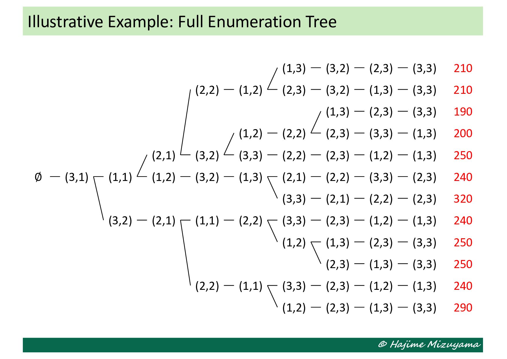
19. © Hajime Mizuyama Illustrative Example: Full Enumeration Tree ∅ (3,1) (1,1) (3,2) (2,1) (2,1) (1,2) (2,2) (3,2) (3,2) (1,1) (2,2) (1,2) (1,3) (3,2) (2,3) (3,3) 210 (2,3) (3,2) (3,3) (1,3) 210 (1,2) (3,3) (2,2) (2,2) (1,3) (2,3) (2,3) (2,3) (3,3) (1,2) (3,3) (1,3) (1,3) 190 200 250 (1,3) (2,1) (3,3) (2,2) (2,1) (3,3) (2,2) (2,3) (2,3) 240 320 (2,2) (1,1) (3,3) (3,3) (1,3) (2,3) (2,3) (2,3) (1,2) (1,2) (1,3) (1,3) (2,3) (1,3) (1,3) (3,3) (1,2) (3,3) (3,3) (1,2) (2,3) 240 250 250 240 290
20. © Hajime Mizuyama Partial Schedules, Partial Precedence Diagrams, and LBs J3 M1 M2 M3 Partial schedule: 𝒔 = ( 3,1 , 1,1 , 1,2 ) J1 J3 M1 M2 M3 Partial schedule: 𝒔 = ( 3,1 , 1,1 , (2,1)) J2 J1 J1 Start (1,1) (2,1) (3,1) (1,2) (2,2) (3,2) (1,3) (2,3) (3,3) 0 30 40 20 70 40 50 End 20 60 80 Start (1,1) (2,1) (3,1) (1,2) (2,2) (3,2) (1,3) (2,3) (3,3) 0 30 40 20 70 40 50 End 20 60 80 0 30 100 0 100 140 30 100 240 180 0 40 0 0 110 40 30 80 160 80 𝐿𝐵(𝒔) = 160 𝐿𝐵(𝒔) = 240
21. © Hajime Mizuyama Partial Enumeration Tree with LBs ∅ (3,1) (1,1) (3,2) (2,1) (1,2) J3 M1 M2 M3 Partial schedule: 𝒔 = ( 3,1 , 1,1 , 1,2 ) J1 J3 M1 M2 M3 Partial schedule: 𝒔 = ( 3,1 , 1,1 , (2,1)) J2 J1 J1 𝐿𝐵(𝒔) = 160 𝐿𝐵(𝒔) = 240 240 80 150 160 190 160
22. © Hajime Mizuyama Enumeration Tree Constructed by BAB ∅ (3,1) (1,1) (3,2) (2,1) (2,1) (1,2) (2,2) (3,2) (1,1) (2,2) (1,2) (3,3) (2,2) (1,3) (2,3) (2,3) (3,3) 190 160 240 80 150 160 190 180 210 190 250 190 190 190 200 200 230 190