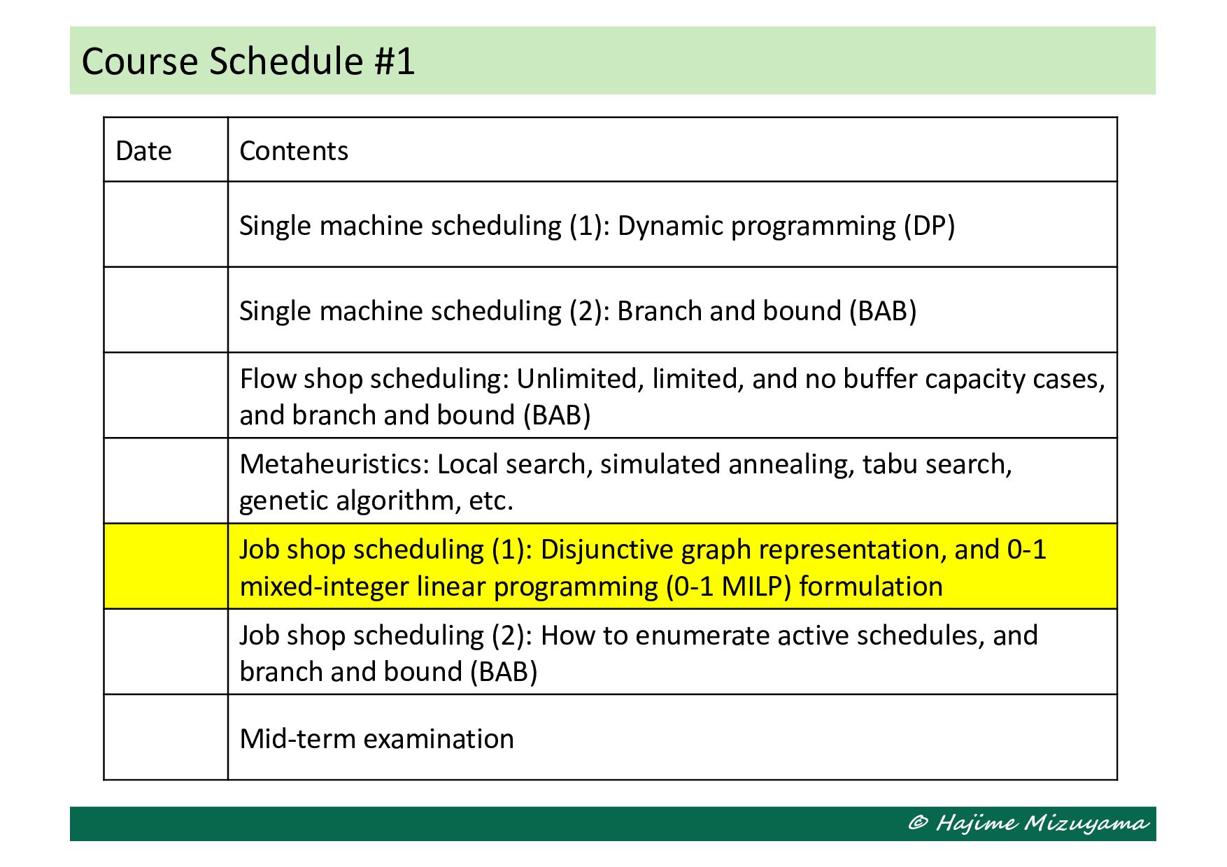
scheduling (1): Dynamic programming (DP) Single machine scheduling (2): Branch and bound (BAB) Flow shop scheduling: Unlimited, limited, and no buffer capacity cases, and branch and bound (BAB) Metaheuristics: Local search, simulated annealing, tabu search, genetic algorithm, etc. Job shop scheduling (1): Disjunctive graph representation, and 0-1 mixed-integer linear programming (0-1 MILP) formulation Job shop scheduling (2): How to enumerate active schedules, and branch and bound (BAB) Mid-term examination
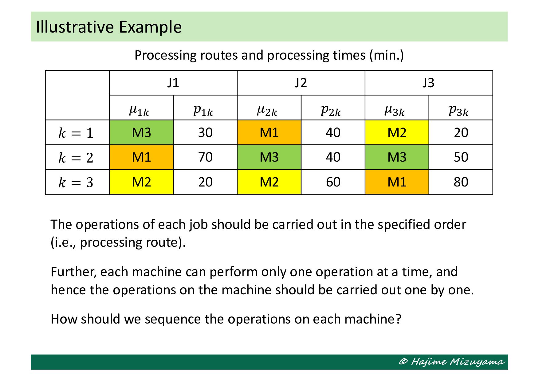
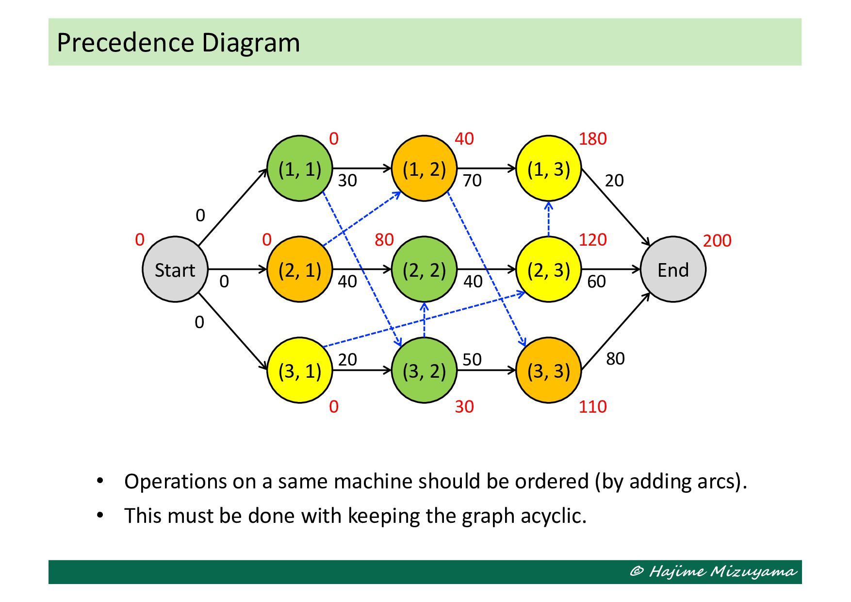
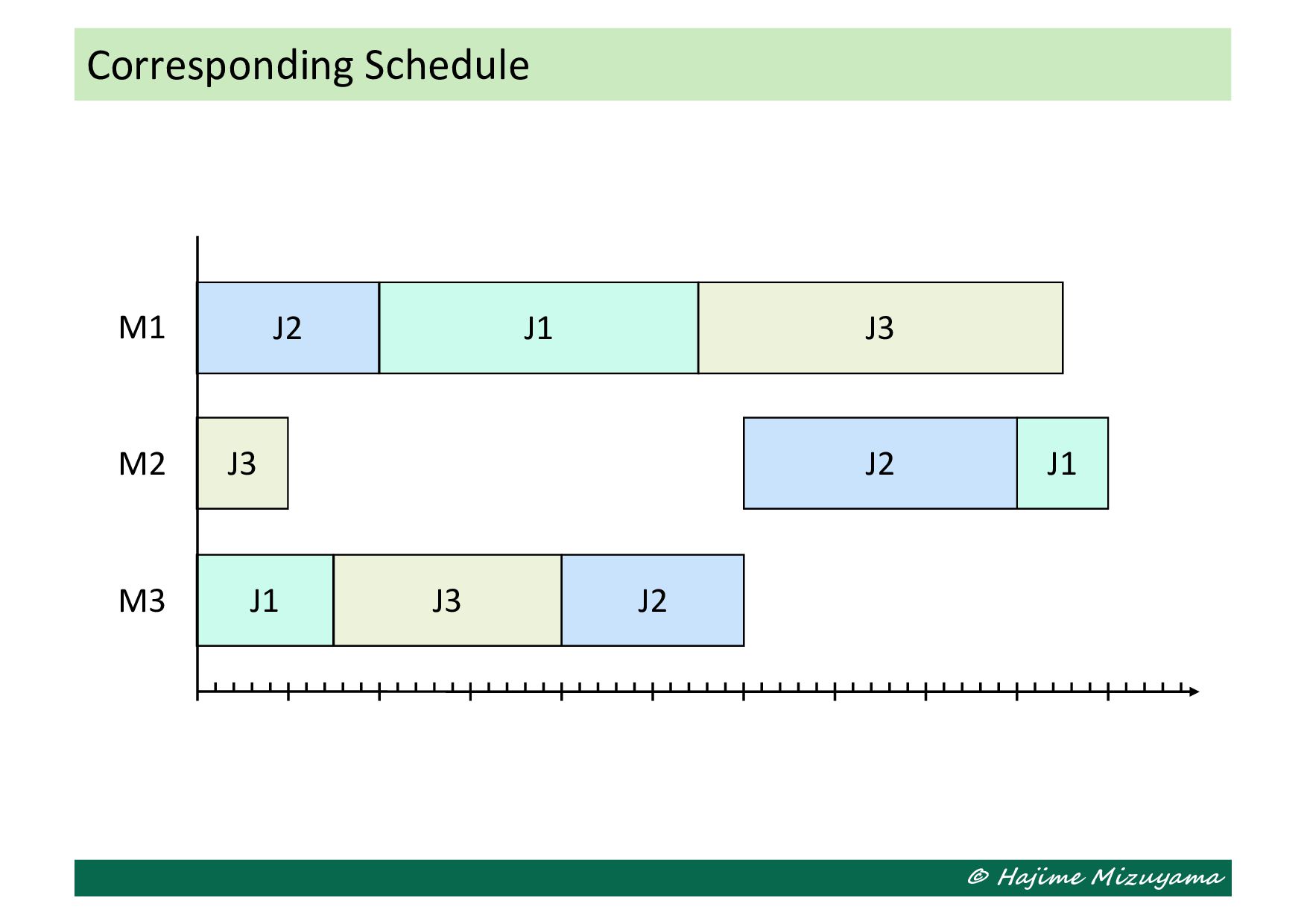
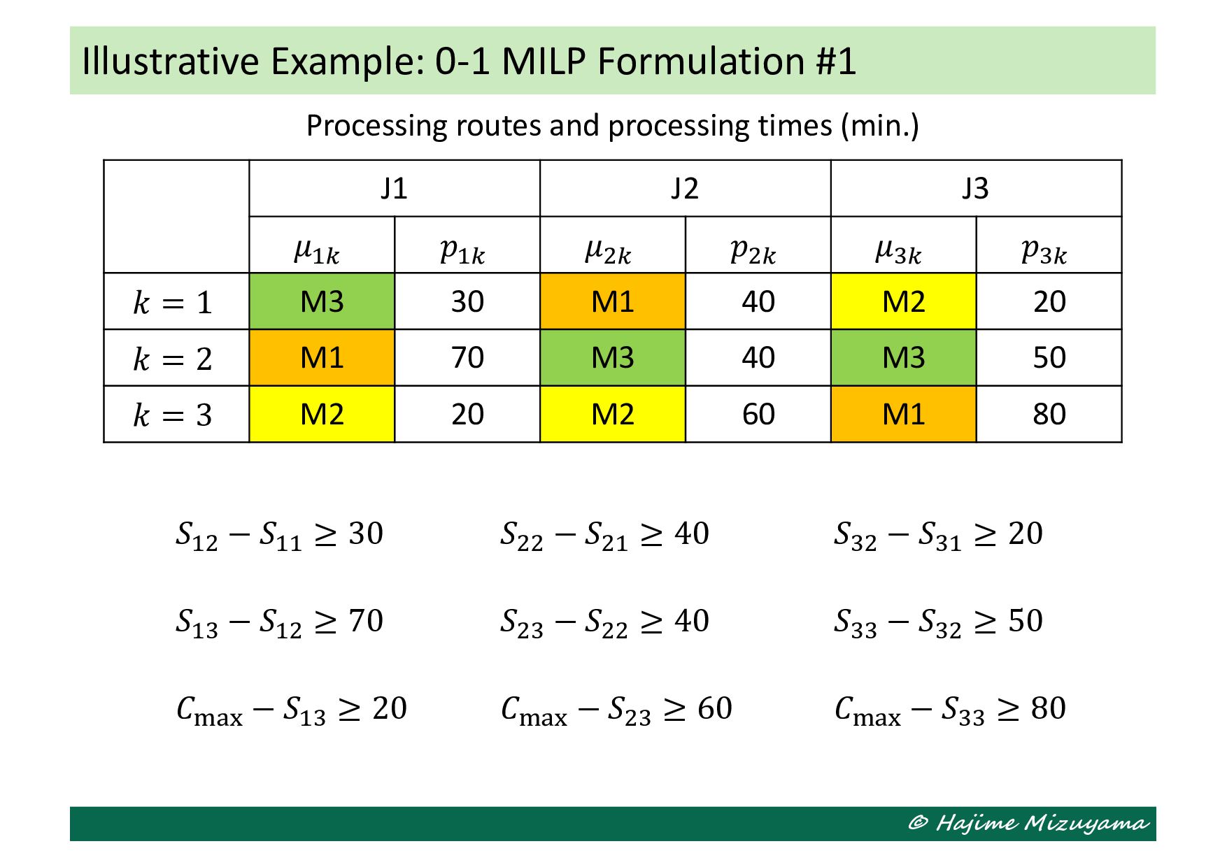
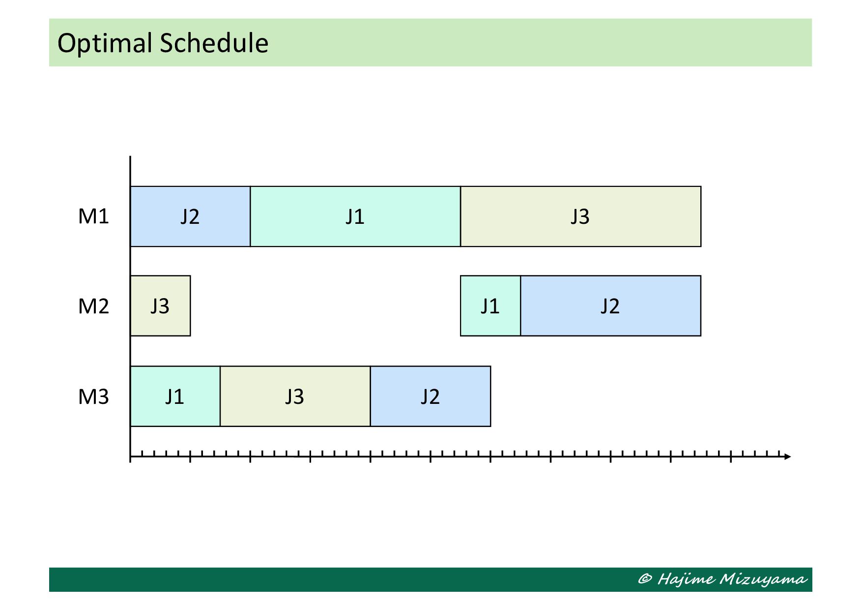
𝜇0# 𝑝0# 𝑘 = 1 M3 30 M1 40 M2 20 𝑘 = 2 M1 70 M3 40 M3 50 𝑘 = 3 M2 20 M2 60 M1 80 Illustrative Example Processing routes and processing times (min.) The operations of each job should be carried out in the specified order (i.e., processing route). Further, each machine can perform only one operation at a time, and hence the operations on the machine should be carried out one by one. How should we sequence the operations on each machine?
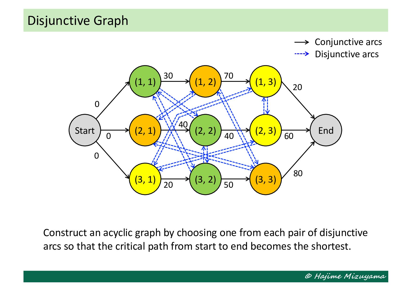
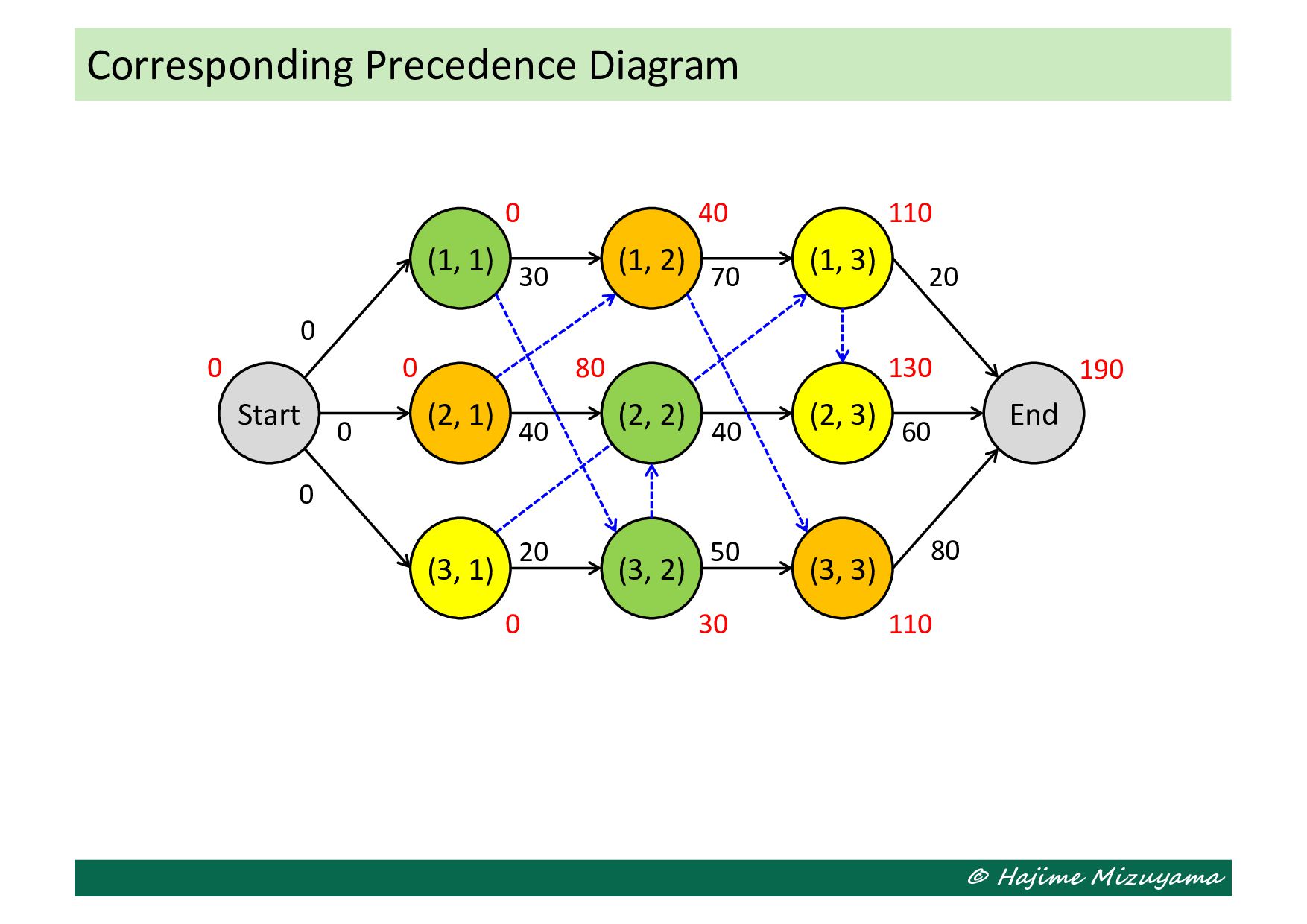
(3, 1) (1, 2) (2, 2) (3, 2) (1, 3) (2, 3) (3, 3) 0 0 0 30 40 20 70 40 50 End 20 60 80 Construct an acyclic graph by choosing one from each pair of disjunctive arcs so that the critical path from start to end becomes the shortest. Conjunctive arcs Disjunctive arcs
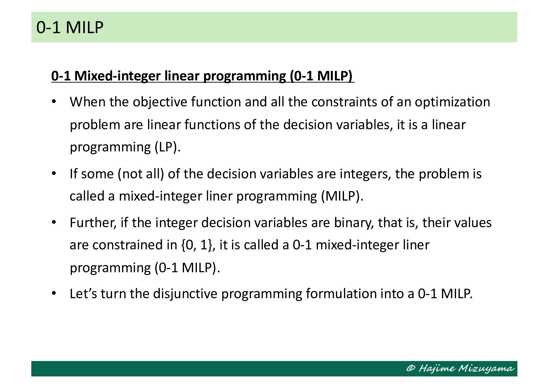
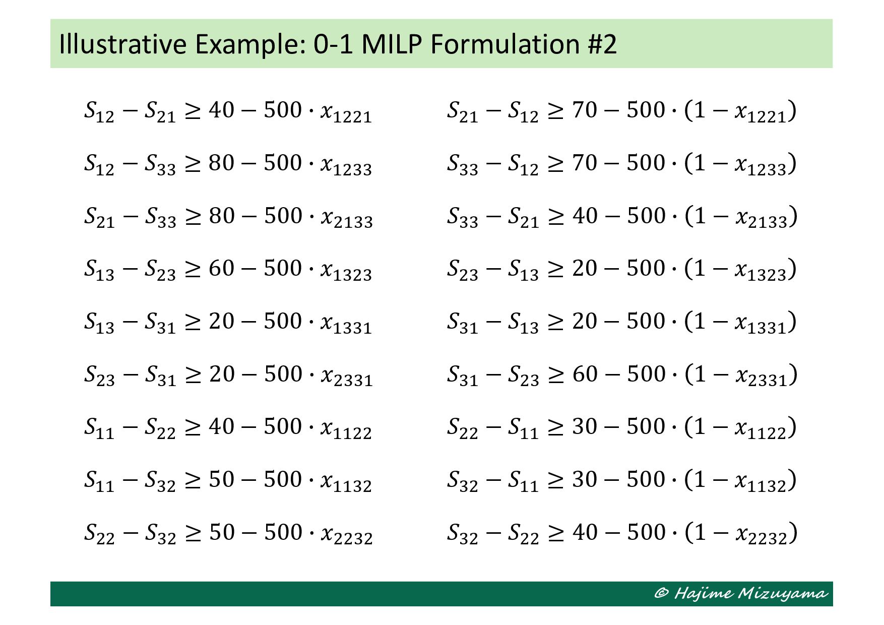
When the objective function and all the constraints of an optimization problem are linear functions of the decision variables, it is a linear programming (LP). • If some (not all) of the decision variables are integers, the problem is called a mixed-integer liner programming (MILP). • Further, if the integer decision variables are binary, that is, their values are constrained in {0, 1}, it is called a 0-1 mixed-integer liner programming (0-1 MILP). • Let’s turn the disjunctive programming formulation into a 0-1 MILP. 0-1 MILP
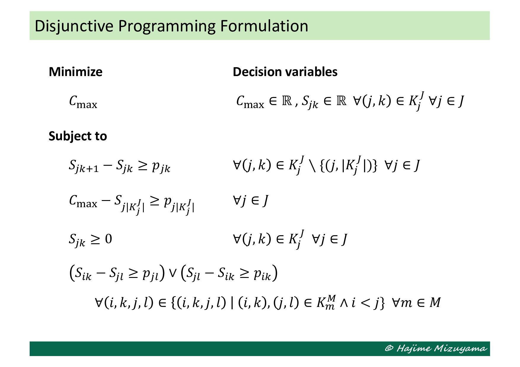
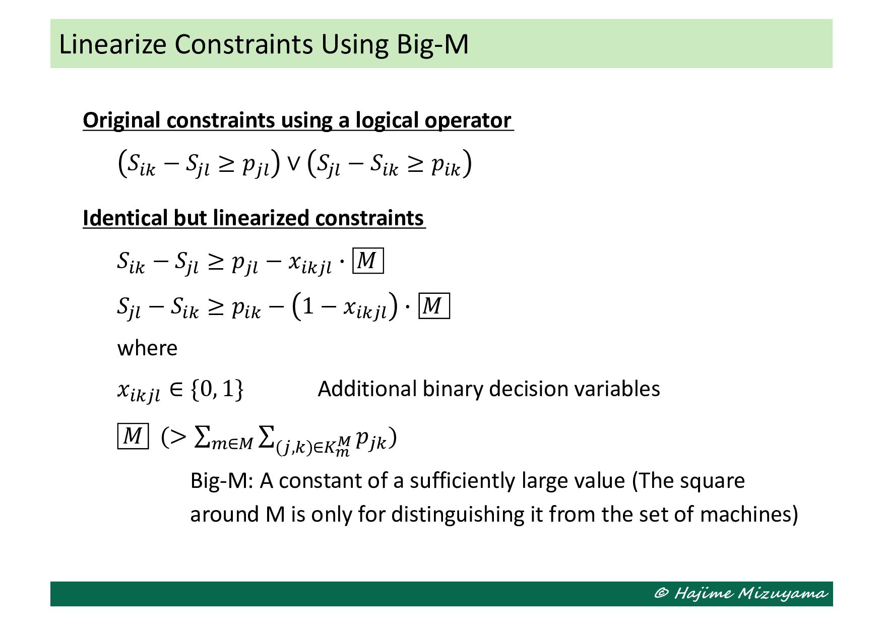
− 𝑆!4 ≥ 𝑝!4 ∨ 𝑆!4 − 𝑆3# ≥ 𝑝3# Identical but linearized constraints 𝑆3# − 𝑆!4 ≥ 𝑝!4 − 𝑥3#!4 H 𝑀 𝑆!4 − 𝑆3# ≥ 𝑝3# − 1 − 𝑥3#!4 H 𝑀 where 𝑥3#!4 ∈ {0, 1} Additional binary decision variables 𝑀 (> ∑$∈% ∑ (!,#)∈(! " 𝑝!# ) Big-M: A constant of a sufficiently large value (The square around M is only for distinguishing it from the set of machines) Linearize Constraints Using Big-M
MILP problems using PuLP (a Python library) and accompanying free solver CBC is available from the following link. Push “Open in Colab” button, then you can test it in Google Colaboratory environment. https://github.com/j54854/myColab/blob/main/pom2_6.ipynb How to Solve 0-1 MILP with PuLP (& CBC Solver)