Lecture slides for POM 2-9

生産管理技術2の講義9のスライドです．

Transcript

1. © Hajime Mizuyama Production & Operations Management #2 @AGU Lec.9: Dynamic Scheduling and Control #1 • Static and dynamic scheduling environments • Discrete-event simulation (DES) • Online job shop scheduling example
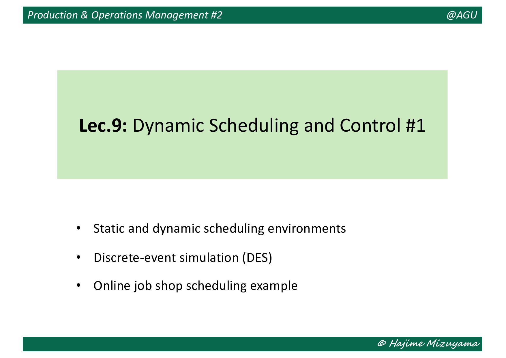
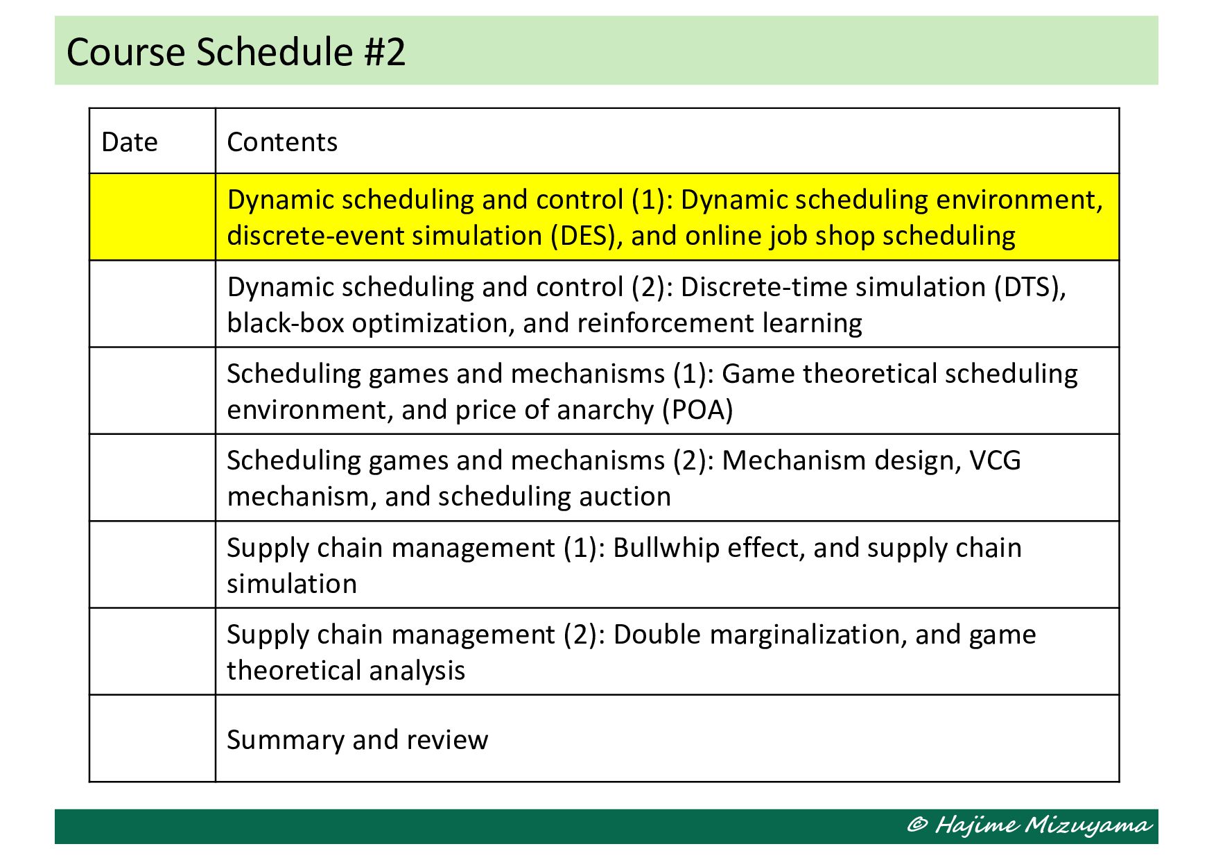
2. © Hajime Mizuyama Course Schedule #2 Date Contents Dynamic scheduling and control (1): Dynamic scheduling environment, discrete-event simulation (DES), and online job shop scheduling Dynamic scheduling and control (2): Discrete-time simulation (DTS), black-box optimization, and reinforcement learning Scheduling games and mechanisms (1): Game theoretical scheduling environment, and price of anarchy (POA) Scheduling games and mechanisms (2): Mechanism design, VCG mechanism, and scheduling auction Supply chain management (1): Bullwhip effect, and supply chain simulation Supply chain management (2): Double marginalization, and game theoretical analysis Summary and review
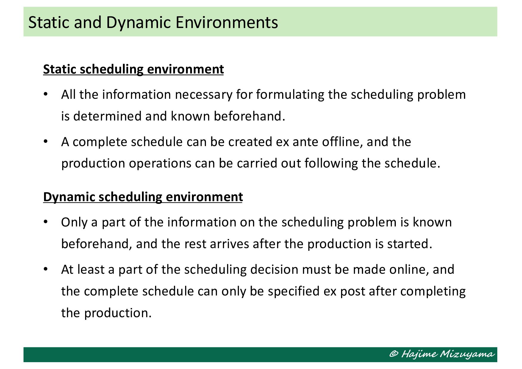
3. © Hajime Mizuyama Static scheduling environment • All the information necessary for formulating the scheduling problem is determined and known beforehand. • A complete schedule can be created ex ante offline, and the production operations can be carried out following the schedule. Dynamic scheduling environment • Only a part of the information on the scheduling problem is known beforehand, and the rest arrives after the production is started. • At least a part of the scheduling decision must be made online, and the complete schedule can only be specified ex post after completing the production. Static and Dynamic Environments
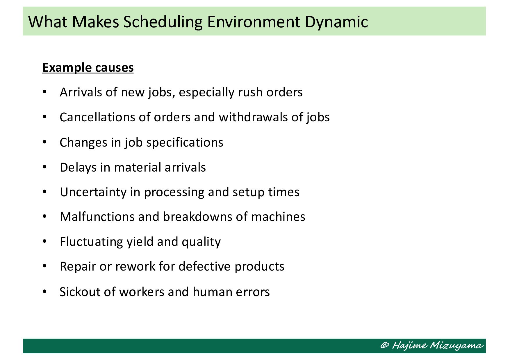
4. © Hajime Mizuyama Example causes • Arrivals of new jobs, especially rush orders • Cancellations of orders and withdrawals of jobs • Changes in job specifications • Delays in material arrivals • Uncertainty in processing and setup times • Malfunctions and breakdowns of machines • Fluctuating yield and quality • Repair or rework for defective products • Sickout of workers and human errors What Makes Scheduling Environment Dynamic
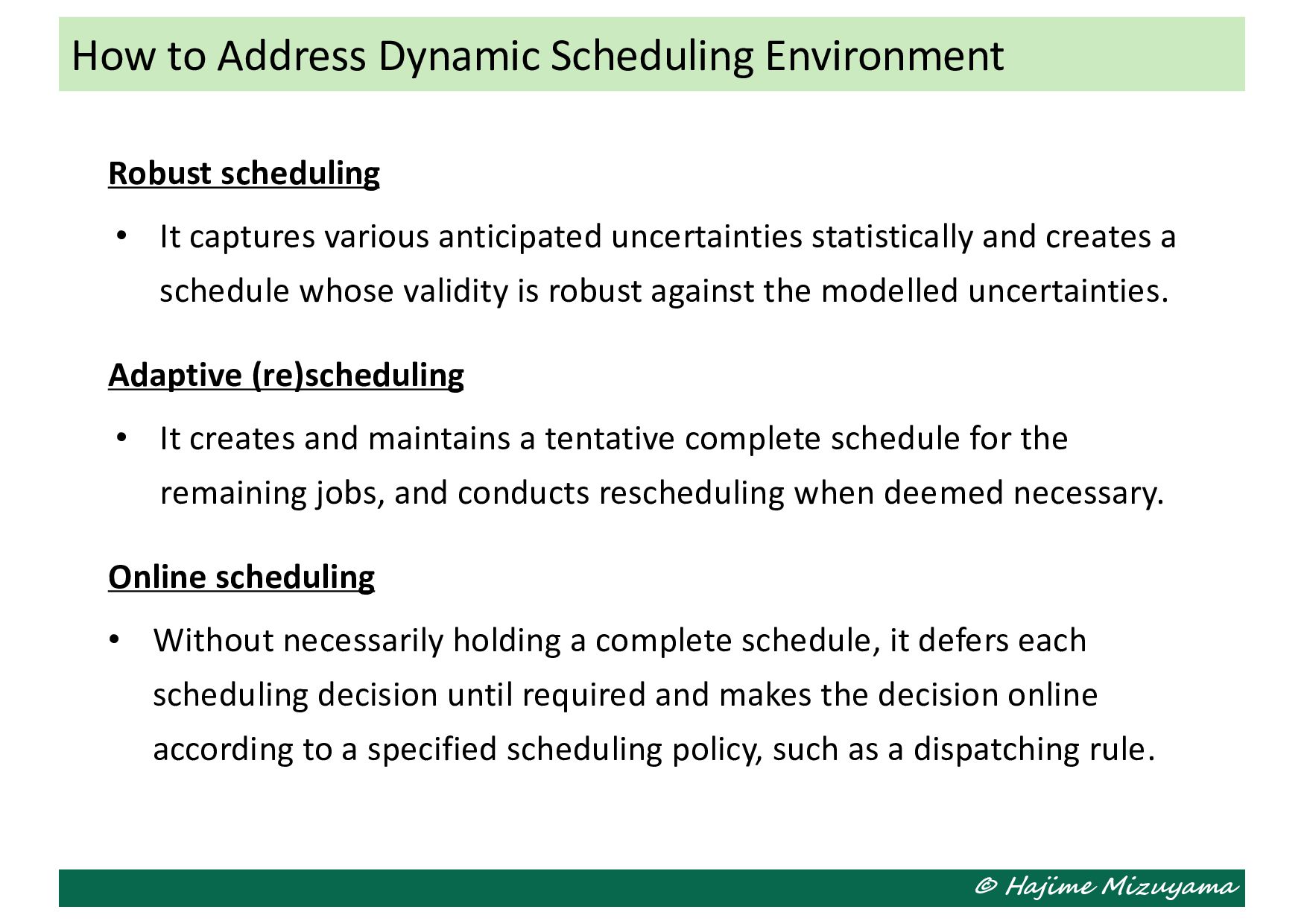
5. © Hajime Mizuyama Robust scheduling • It captures various anticipated uncertainties statistically and creates a schedule whose validity is robust against the modelled uncertainties. Adaptive (re)scheduling • It creates and maintains a tentative complete schedule for the remaining jobs, and conducts rescheduling when deemed necessary. Online scheduling • Without necessarily holding a complete schedule, it defers each scheduling decision until required and makes the decision online according to a specified scheduling policy, such as a dispatching rule. How to Address Dynamic Scheduling Environment
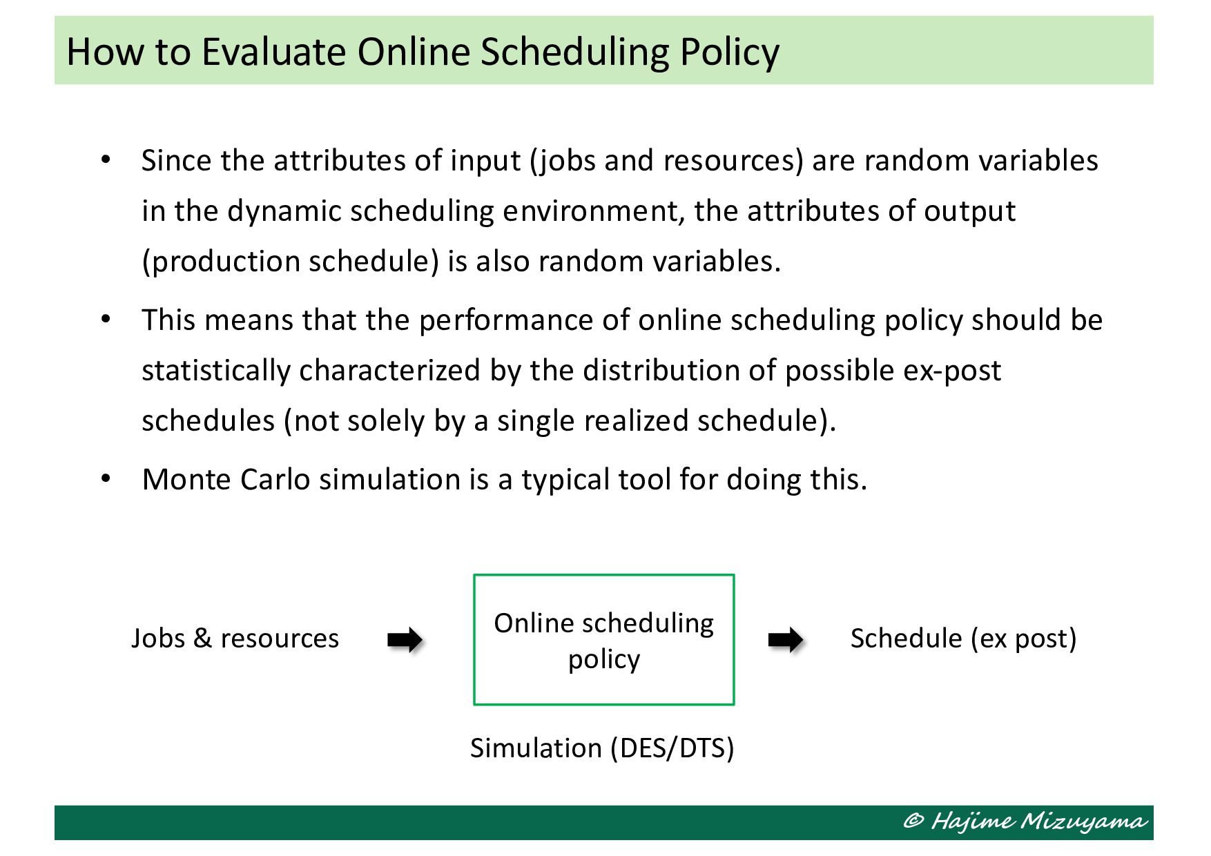
6. © Hajime Mizuyama • Since the attributes of input (jobs and resources) are random variables in the dynamic scheduling environment, the attributes of output (production schedule) is also random variables. • This means that the performance of online scheduling policy should be statistically characterized by the distribution of possible ex-post schedules (not solely by a single realized schedule). • Monte Carlo simulation is a typical tool for doing this. How to Evaluate Online Scheduling Policy Online scheduling policy Jobs & resources Schedule (ex post) Simulation (DES/DTS)
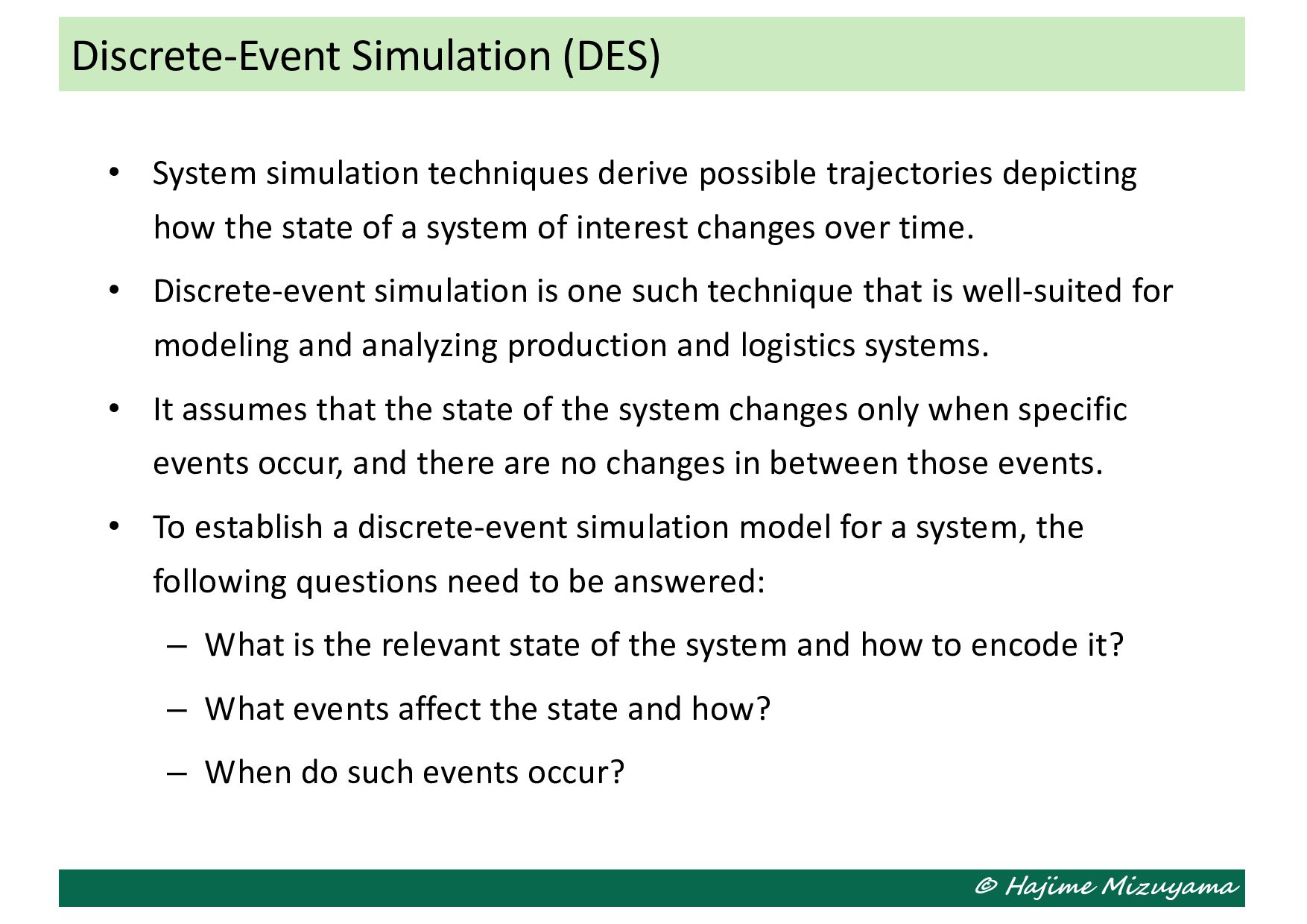
7. © Hajime Mizuyama • System simulation techniques derive possible trajectories depicting how the state of a system of interest changes over time. • Discrete-event simulation is one such technique that is well-suited for modeling and analyzing production and logistics systems. • It assumes that the state of the system changes only when specific events occur, and there are no changes in between those events. • To establish a discrete-event simulation model for a system, the following questions need to be answered: – What is the relevant state of the system and how to encode it? – What events affect the state and how? – When do such events occur? Discrete-Event Simulation (DES)
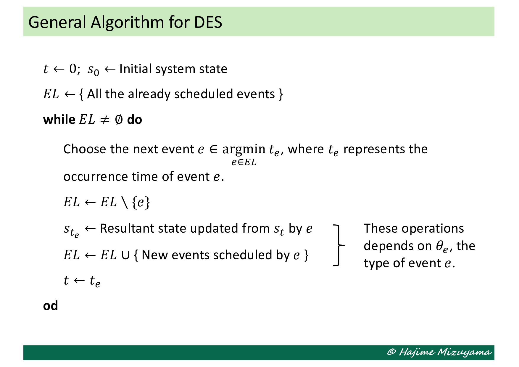
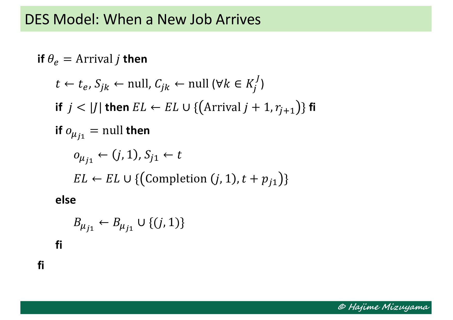
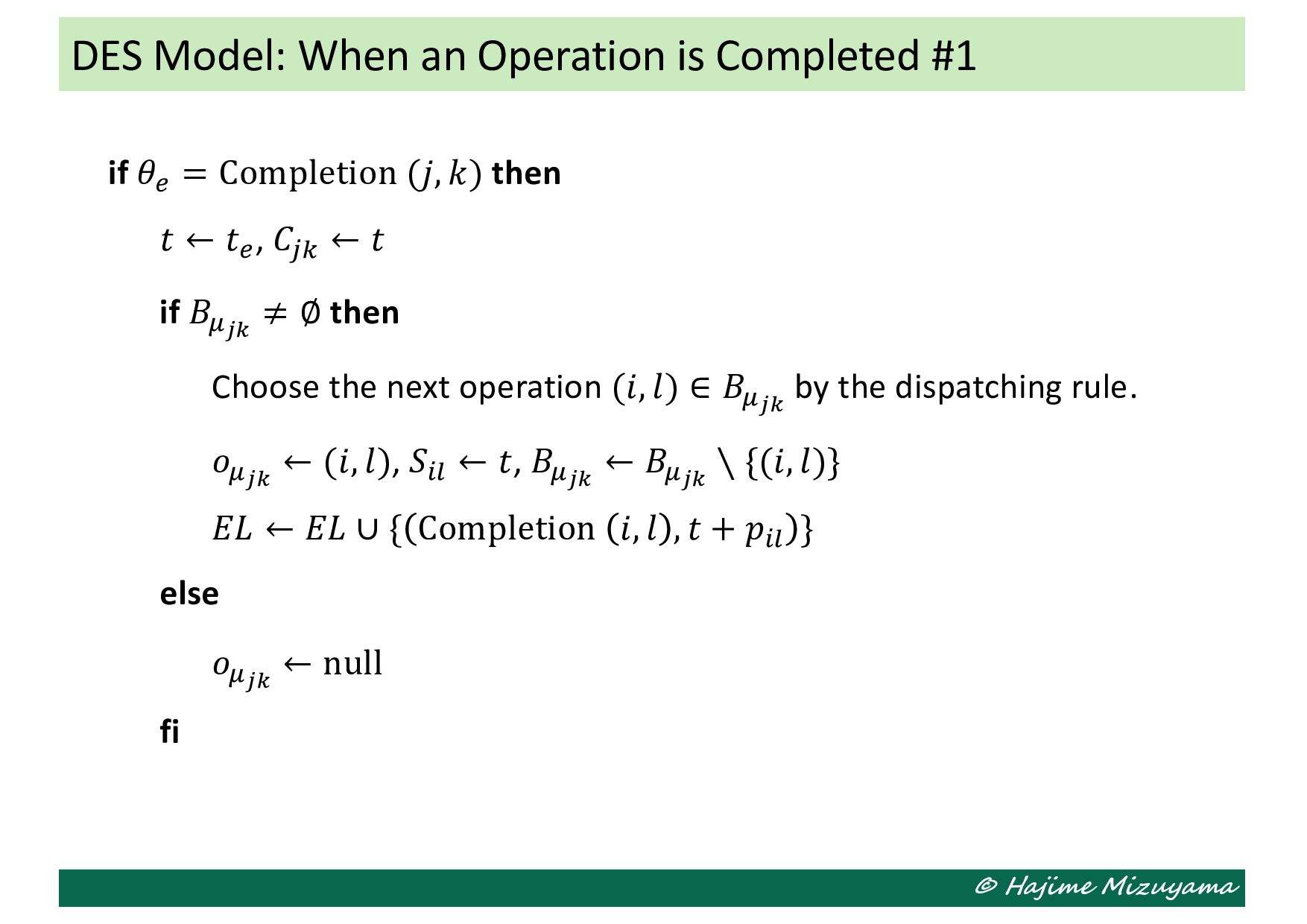
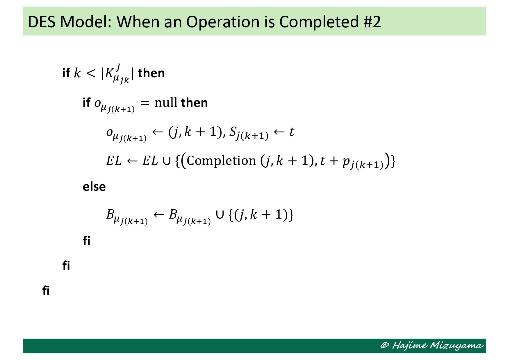
8. © Hajime Mizuyama 𝑡 ← 0; 𝑠! ← Initial system state 𝐸𝐿 ← { All the already scheduled events } while 𝐸𝐿 ≠ ∅ do Choose the next event 𝑒 ∈ argmin "∈$% 𝑡", where 𝑡" represents the occurrence time of event 𝑒. 𝐸𝐿 ← 𝐸𝐿 ∖ {𝑒} 𝑠&! ← Resultant state updated from 𝑠& by 𝑒 𝐸𝐿 ← 𝐸𝐿 ∪ { New events scheduled by 𝑒 } 𝑡 ← 𝑡" od General Algorithm for DES These operations depends on 𝜃", the type of event 𝑒.
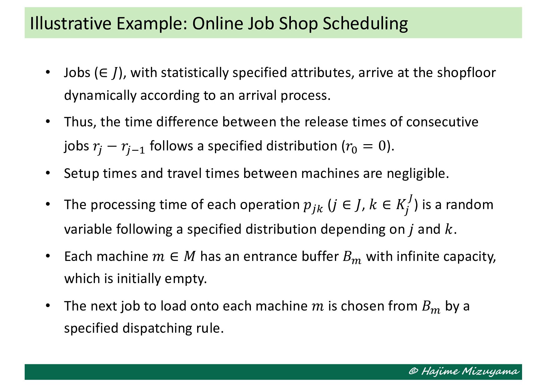
9. © Hajime Mizuyama • Jobs (∈ 𝐽), with statistically specified attributes, arrive at the shopfloor dynamically according to an arrival process. • Thus, the time difference between the release times of consecutive jobs 𝑟' − 𝑟'() follows a specified distribution (𝑟! = 0). • Setup times and travel times between machines are negligible. • The processing time of each operation 𝑝'* (𝑗 ∈ 𝐽, 𝑘 ∈ 𝐾' + ) is a random variable following a specified distribution depending on 𝑗 and 𝑘. • Each machine 𝑚 ∈ 𝑀 has an entrance buffer 𝐵, with infinite capacity, which is initially empty. • The next job to load onto each machine 𝑚 is chosen from 𝐵, by a specified dispatching rule. Illustrative Example: Online Job Shop Scheduling
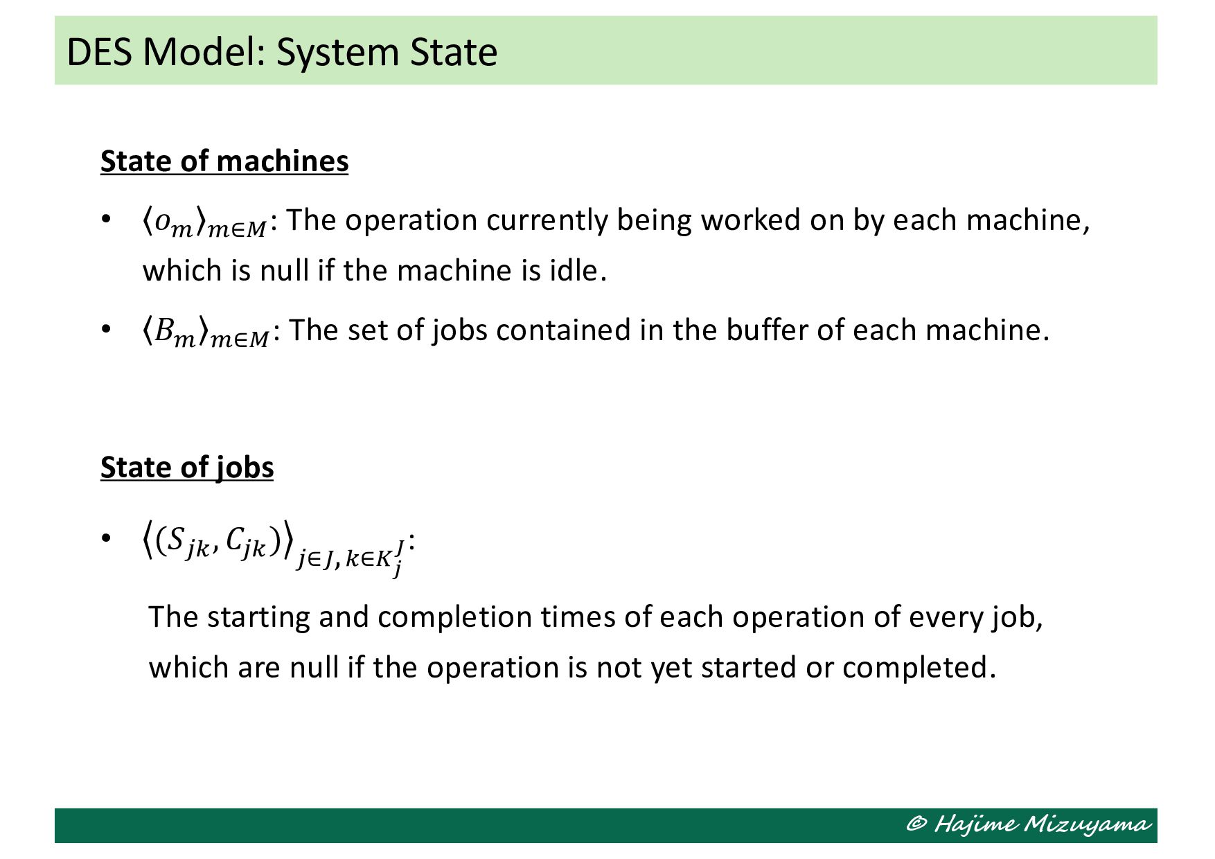
10. © Hajime Mizuyama State of machines • 𝑜, ,∈-: The operation currently being worked on by each machine, which is null if the machine is idle. • 𝐵, ,∈-: The set of jobs contained in the buffer of each machine. State of jobs • (𝑆'* , 𝐶'* ) '∈+,*∈." # : The starting and completion times of each operation of every job, which are null if the operation is not yet started or completed. DES Model: System State
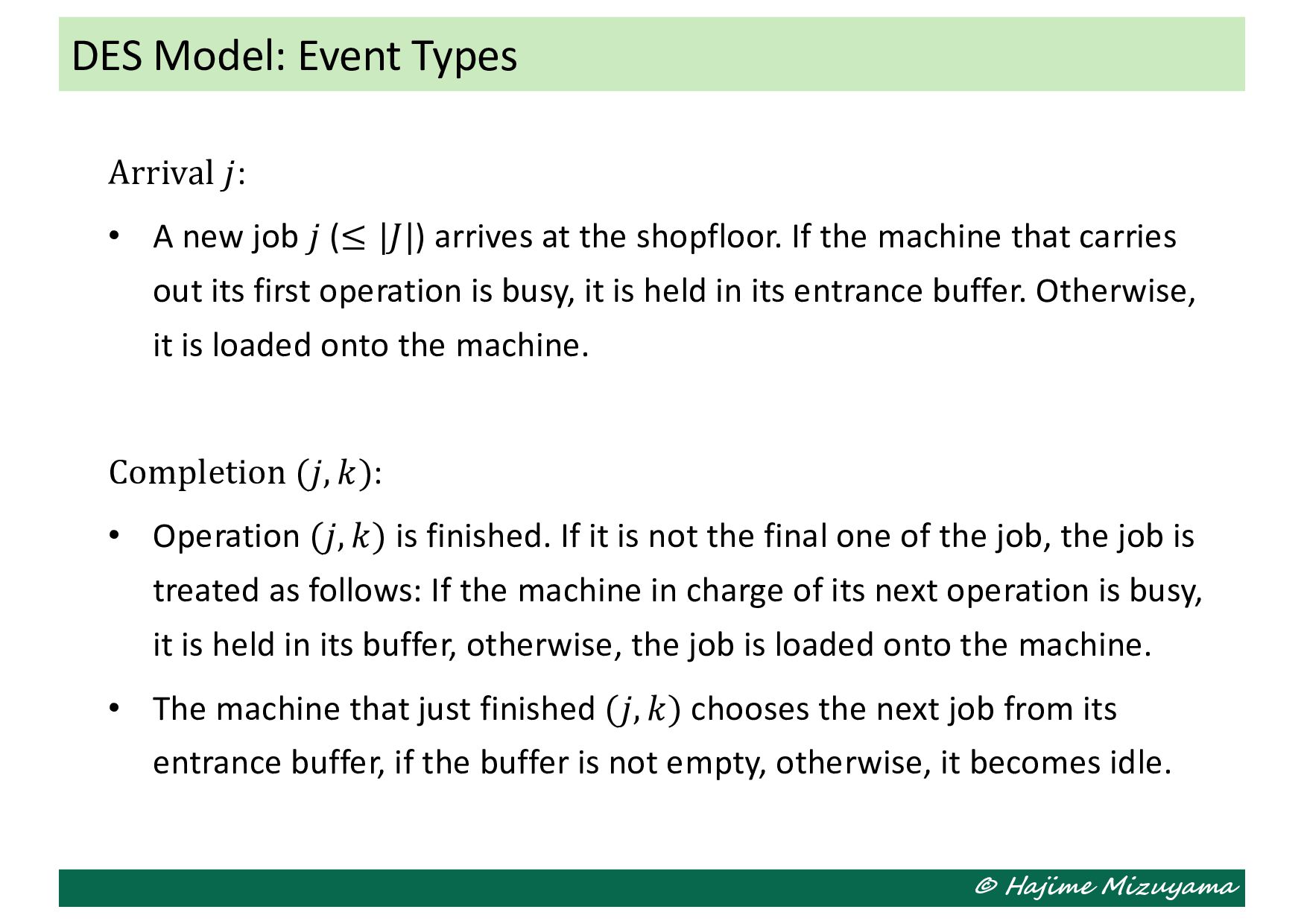
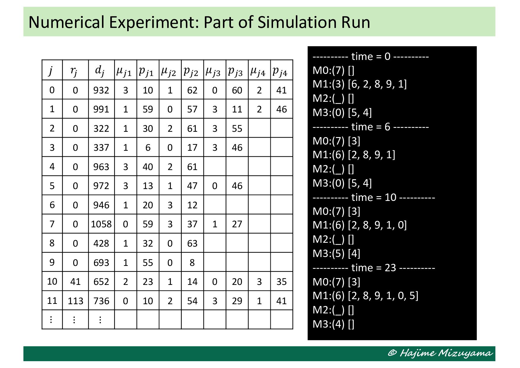
11. © Hajime Mizuyama Arrival 𝑗: • A new job 𝑗 (≤ |𝐽|) arrives at the shopfloor. If the machine that carries out its first operation is busy, it is held in its entrance buffer. Otherwise, it is loaded onto the machine. Completion (𝑗, 𝑘): • Operation (𝑗, 𝑘) is finished. If it is not the final one of the job, the job is treated as follows: If the machine in charge of its next operation is busy, it is held in its buffer, otherwise, the job is loaded onto the machine. • The machine that just finished (𝑗, 𝑘) chooses the next job from its entrance buffer, if the buffer is not empty, otherwise, it becomes idle. DES Model: Event Types
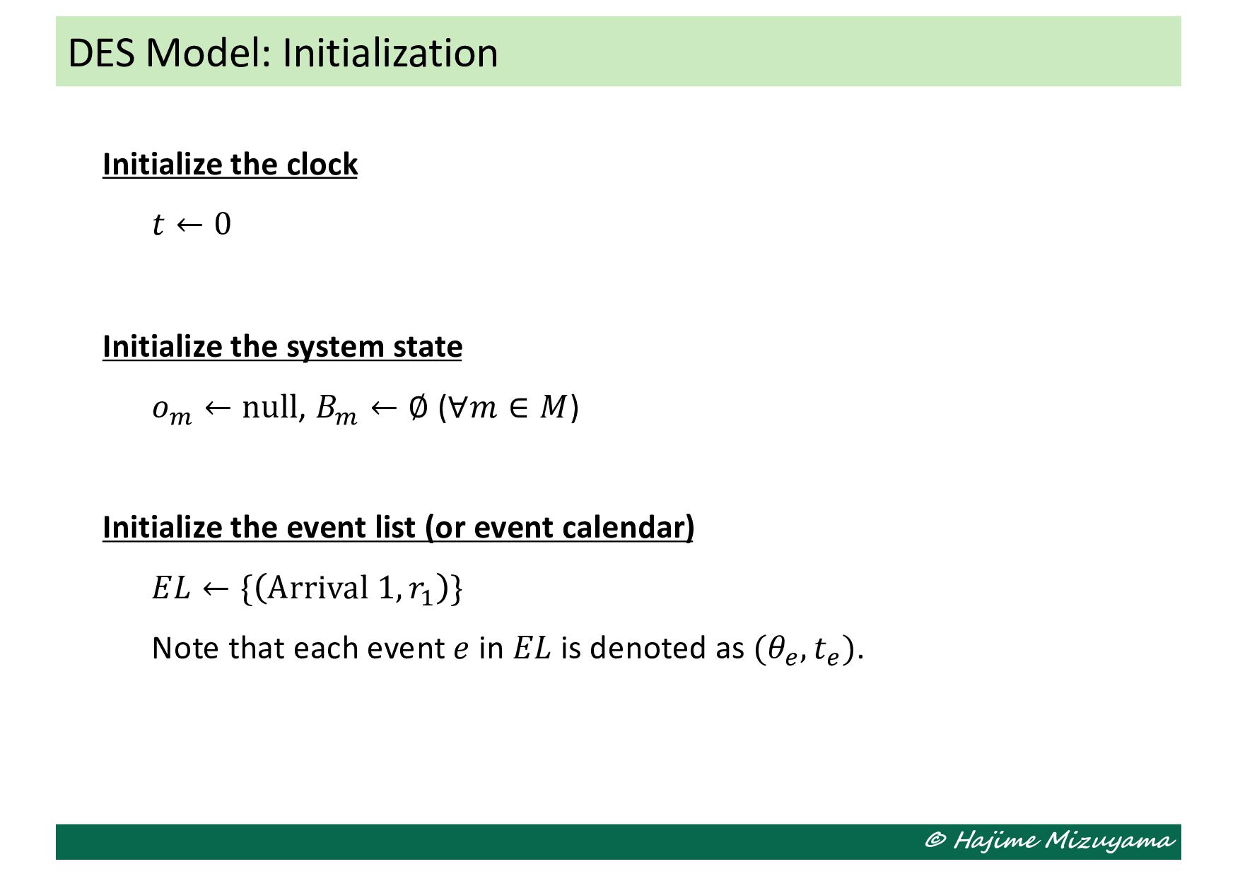
12. © Hajime Mizuyama Initialize the clock 𝑡 ← 0 Initialize the system state 𝑜, ← null, 𝐵, ← ∅ (∀𝑚 ∈ 𝑀) Initialize the event list (or event calendar) 𝐸𝐿 ← { Arrival 1, 𝑟) } Note that each event 𝑒 in 𝐸𝐿 is denoted as (𝜃" , 𝑡" ). DES Model: Initialization
13. © Hajime Mizuyama if 𝜃" = Arrival 𝑗 then 𝑡 ← 𝑡", 𝑆'* ← null, 𝐶'* ← null (∀𝑘 ∈ 𝐾' + ) if 𝑗 < |𝐽| then 𝐸𝐿 ← 𝐸𝐿 ∪ { Arrival 𝑗 + 1, 𝑟'/) } fi if 𝑜0"$ = null then 𝑜0"$ ← 𝑗, 1 , 𝑆') ← 𝑡 𝐸𝐿 ← 𝐸𝐿 ∪ { Completion 𝑗, 1 , 𝑡 + 𝑝') } else 𝐵0"$ ← 𝐵0"$ ∪ {(𝑗, 1)} fi fi DES Model: When a New Job Arrives
14. © Hajime Mizuyama if 𝜃" = Completion (𝑗, 𝑘) then 𝑡 ← 𝑡", 𝐶'* ← 𝑡 if 𝐵0"% ≠ ∅ then Choose the next operation (𝑖, 𝑙) ∈ 𝐵0"% by the dispatching rule. 𝑜0"% ← (𝑖, 𝑙), 𝑆12 ← 𝑡, 𝐵0"% ← 𝐵0"% ∖ {(𝑖, 𝑙)} 𝐸𝐿 ← 𝐸𝐿 ∪ { Completion 𝑖, 𝑙 , 𝑡 + 𝑝12 } else 𝑜0"% ← null fi DES Model: When an Operation is Completed #1
15. © Hajime Mizuyama if 𝑘 < |𝐾0"% + | then if 𝑜0"(%'$) = null then 𝑜0"(%'$) ← (𝑗, 𝑘 + 1), 𝑆'(*/)) ← 𝑡 𝐸𝐿 ← 𝐸𝐿 ∪ { Completion 𝑗, 𝑘 + 1 , 𝑡 + 𝑝'(*/)) } else 𝐵0"(%'$) ← 𝐵0"(%'$) ∪ {(𝑗, 𝑘 + 1)} fi fi fi DES Model: When an Operation is Completed #2
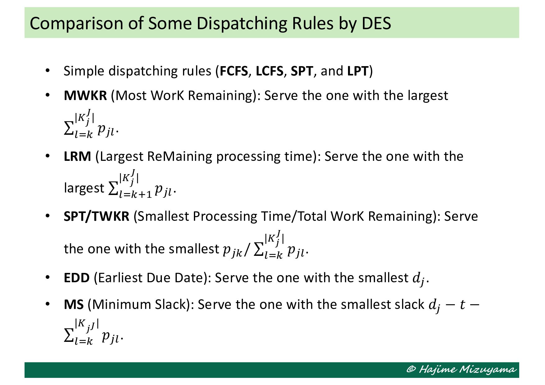
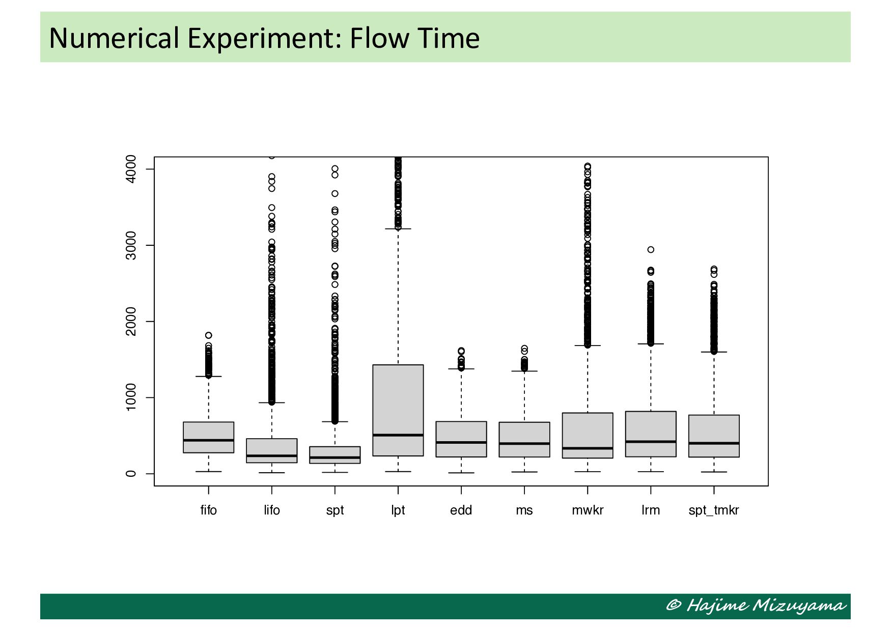
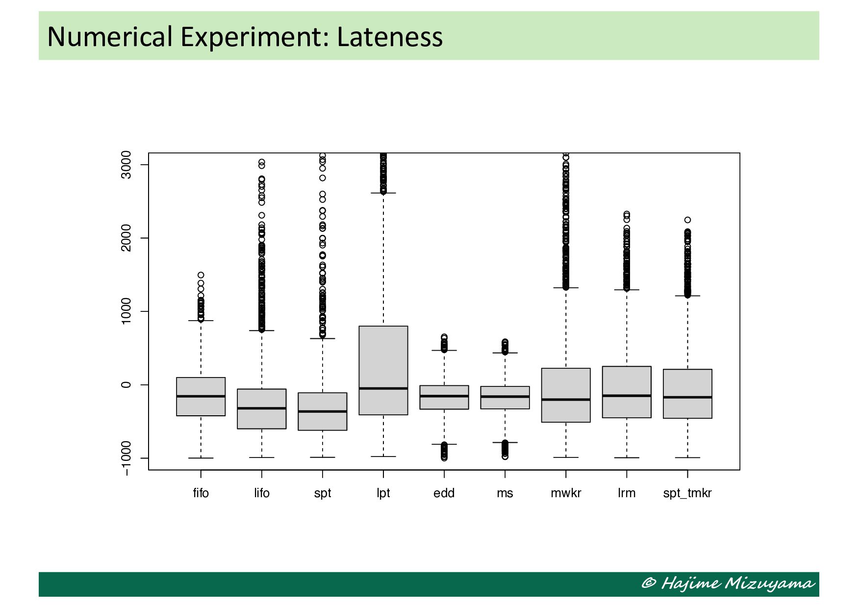
16. © Hajime Mizuyama • Simple dispatching rules (FCFS, LCFS, SPT, and LPT) • MWKR (Most WorK Remaining): Serve the one with the largest ∑ 25* |." #| 𝑝'2. • LRM (Largest ReMaining processing time): Serve the one with the largest ∑ 25*/) |." # | 𝑝'2. • SPT/TWKR (Smallest Processing Time/Total WorK Remaining): Serve the one with the smallest 𝑝'* / ∑ 25* |." #| 𝑝'2. • EDD (Earliest Due Date): Serve the one with the smallest 𝑑'. • MS (Minimum Slack): Serve the one with the smallest slack 𝑑' − 𝑡 − ∑ 25* |. "#| 𝑝'2. Comparison of Some Dispatching Rules by DES
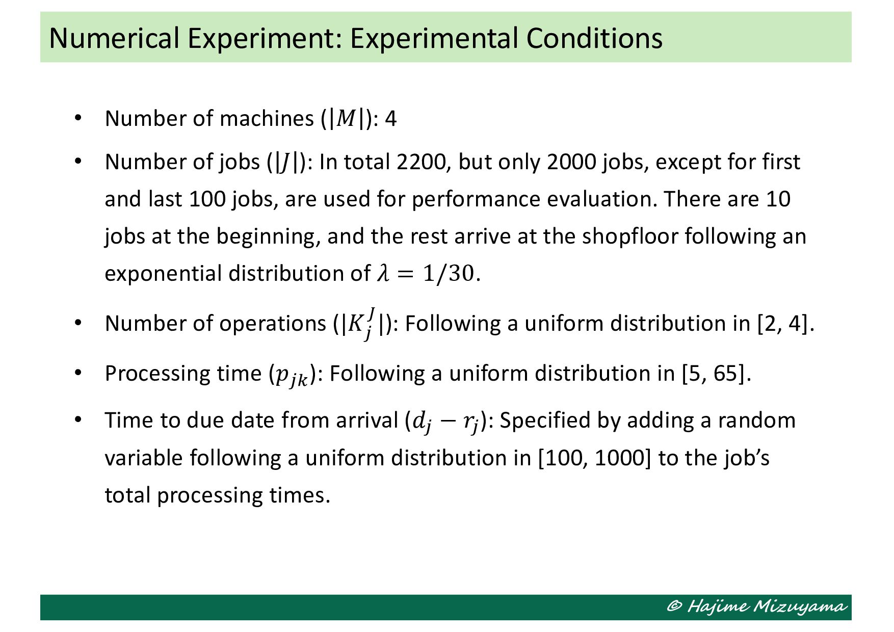
17. © Hajime Mizuyama • Number of machines ( 𝑀 ): 4 • Number of jobs ( 𝐽 ): In total 2200, but only 2000 jobs, except for first and last 100 jobs, are used for performance evaluation. There are 10 jobs at the beginning, and the rest arrive at the shopfloor following an exponential distribution of 𝜆 = 1/30. • Number of operations (|𝐾' +|): Following a uniform distribution in [2, 4]. • Processing time (𝑝'*): Following a uniform distribution in [5, 65]. • Time to due date from arrival (𝑑' − 𝑟'): Specified by adding a random variable following a uniform distribution in [100, 1000] to the job’s total processing times. Numerical Experiment: Experimental Conditions
18. © Hajime Mizuyama Numerical Experiment: Part of Simulation Run 𝑗 𝑟 ) 𝑑) 𝜇)* 𝑝)* 𝜇)+ 𝑝)+ 𝜇), 𝑝), 𝜇)- 𝑝)- 0 0 932 3 10 1 62 0 60 2 41 1 0 991 1 59 0 57 3 11 2 46 2 0 322 1 30 2 61 3 55 3 0 337 1 6 0 17 3 46 4 0 963 3 40 2 61 5 0 972 3 13 1 47 0 46 6 0 946 1 20 3 12 7 0 1058 0 59 3 37 1 27 8 0 428 1 32 0 63 9 0 693 1 55 0 8 10 41 652 2 23 1 14 0 20 3 35 11 113 736 0 10 2 54 3 29 1 41 ⋮ ⋮ ⋮ ---------- time = 0 ---------- M0:(7) [] M1:(3) [6, 2, 8, 9, 1] M2:(_) [] M3:(0) [5, 4] ---------- time = 6 ---------- M0:(7) [3] M1:(6) [2, 8, 9, 1] M2:(_) [] M3:(0) [5, 4] ---------- time = 10 ---------- M0:(7) [3] M1:(6) [2, 8, 9, 1, 0] M2:(_) [] M3:(5) [4] ---------- time = 23 ---------- M0:(7) [3] M1:(6) [2, 8, 9, 1, 0, 5] M2:(_) [] M3:(4) []
19. © Hajime Mizuyama fifo lifo spt lpt edd ms mwkr lrm spt_tmkr 0 1000 2000 3000 4000 Numerical Experiment: Flow Time
20. © Hajime Mizuyama Numerical Experiment: Lateness fifo lifo spt lpt edd ms mwkr lrm spt_tmkr −1000 0 1000 2000 3000
21. © Hajime Mizuyama Supplemental material on how to develop a discrete-event simulator for online job shop scheduling and to compare several dispatching rules on the simulator is available from the following link. Push “Open in Colab” button, then you can test it in Google Colaboratory environment. https://github.com/j54854/myColab/blob/main/pom2_9.ipynb Discrete-Event Simulator for Online Job Shop Scheduling