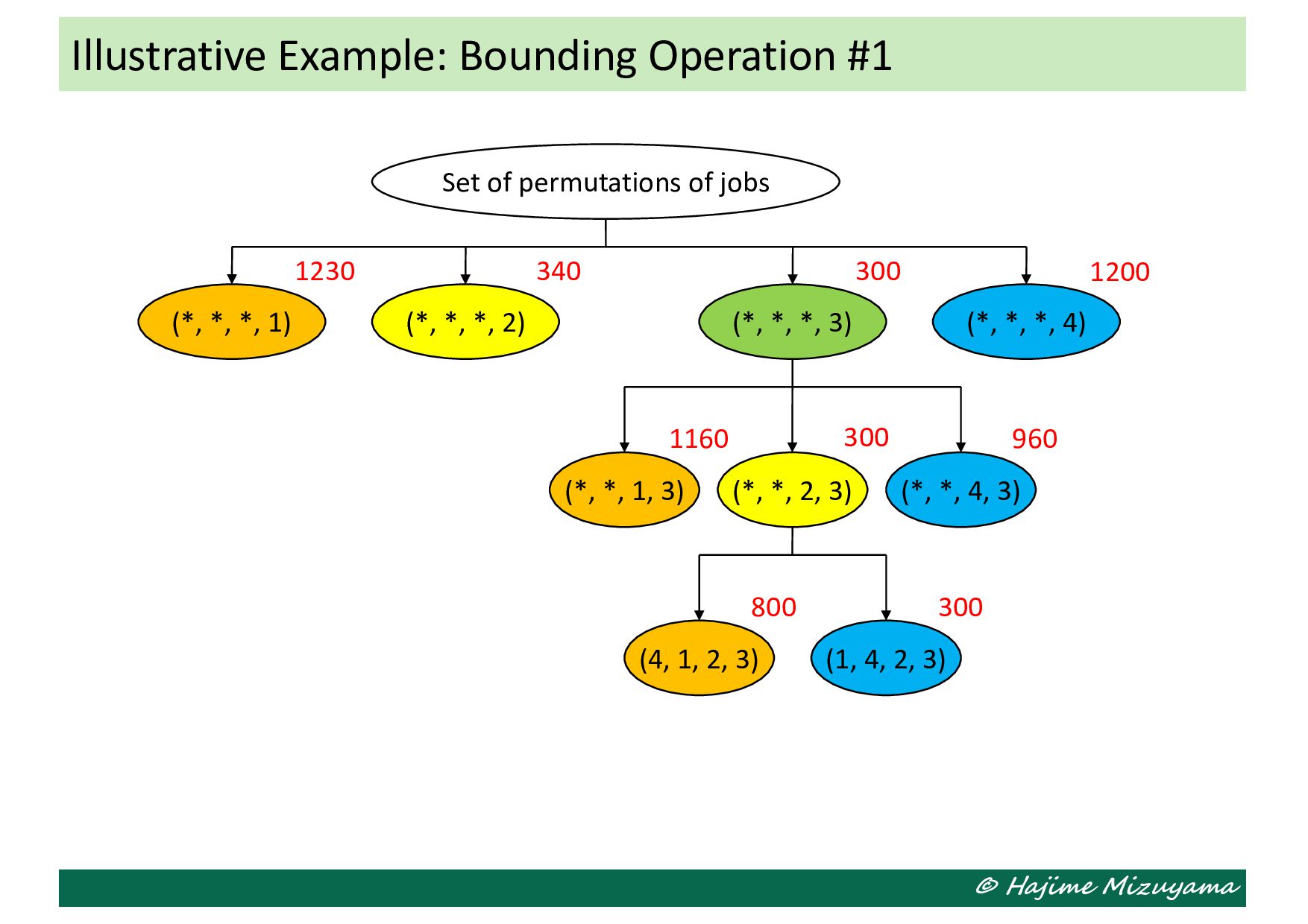
Upgrade to Pro — share decks privately, control downloads, hide ads and more …

Lecture slides for POM 2-2

hajimizu
September 08, 2023

Lecture slides for POM 2-2

生産管理技術2の講義2のスライドです.

hajimizu

September 08, 2023
Tweet

More Decks by hajimizu

Other Decks in Technology

Transcript

  1. © Hajime Mizuyama Production & Operations Management #2 @AGU Lec.2:

    Single Machine Scheduling #1 • Some easily solvable problems (revisited) • Dynamic programming (DP) • DP for minimizing total weighted tardiness
  2. © Hajime Mizuyama Course Schedule #1 Date Contents Single machine

    scheduling (1): Dynamic programming (DP) Single machine scheduling (2): Branch and bound (BAB) Flow shop scheduling: Unlimited, limited, and no buffer capacity cases, and branch and bound (BAB) Metaheuristics: Local search, simulated annealing, tabu search, genetic algorithm, etc. Job shop scheduling (1): Disjunctive graph representation, and 0-1 mixed-integer linear programming (0-1 MILP) formulation Job shop scheduling (2): How to enumerate active schedules, and branch and bound (BAB) Mid-term examination
  3. © Hajime Mizuyama There are only one machine and several

    jobs. The sequence of the jobs 𝜋 should be properly determined to attain a specified objective. • Set of jobs: 𝐽 = {1, 2, … , |𝐽|} • Processing time of job 𝑗 ∈ 𝐽: 𝑝! • Weight of job 𝑗 ∈ 𝐽: 𝑤! • Due date of job 𝑗 ∈ 𝐽: 𝑑! • Set of permutations of jobs in 𝐽: Π" ∋ 𝜋 = 𝜋# , 𝜋$ , … , 𝜋 " • Starting time of job 𝑗 ∈ 𝐽: 𝑆! • Completion time of job 𝑗 ∈ 𝐽: 𝐶! Sigle-Machine Scheduling Problem
  4. © Hajime Mizuyama • Makespan: 𝐶%&' = max !∈" 𝐶!

    – This does not depend on the job sequence 𝜋 in the standard setting considered here. • Total weighted (or unweighted) completion times: ∑!∈" 𝑤! 𝐶! • Maximum weighted (or unweighted) tardiness: max !∈" 𝑤! 𝑇! • Total weighted (or unweighted) tardiness: ∑!∈" 𝑤! 𝑇! – Lateness of job 𝑗 ∈ 𝐽: 𝐿! = 𝐶! − 𝑑! – Tardiness of job 𝑗 ∈ 𝐽: 𝑇! = max(0, 𝐿! ) Typical Objectives
  5. © Hajime Mizuyama Illustrative Example Total completion times ∑!∈" 𝐶!

    = 610 (unweighted) ∑!∈" 𝑤! 𝐶! = 3820 (weighted) Maximum Tardiness max !∈" 𝑇! = 120 (unweighted) max !∈" 𝑤! 𝑇! = 1200 (weighted) Total tardiness ∑!∈" 𝑇! = 140 (unweighted) ∑!∈" 𝑤! 𝑇! = 1240 (weighted) 𝑗 1 2 3 4 𝑝! 40 80 50 110 𝑤! 5 4 2 10 𝑑! 50 220 150 160 𝐶! 40 120 170 280 𝑇 ! 0 0 20 120 𝑑" 𝑑# 𝑑$ 𝑑% If 𝜋 = (1, 2, 3, 4) is used, Example jobs
  6. © Hajime Mizuyama Some Easily Solvable Problems • Total completion

    times – SPT rule • Total weighted completion times – WSPT rule • Maximum tardiness – EDD rule • Maximum weighted tardiness – Simple backward algorithm shown on the right 𝑁 ← 𝐽; 𝑖 ← |𝐽|; E 𝐶 ← ∑!∈" 𝑝! while 𝑁 ≠ 𝜙 do Choose a job ̃ 𝚥 which satisfies: ̃ 𝚥 ∈ argmin !∈) 𝑤! N max(0, E 𝐶 − 𝑑! ) 𝜋* ← ̃ 𝚥; 𝑁 ← 𝑁 ∖ { ̃ 𝚥} E 𝐶 ← E 𝐶 − 𝑝 ̃ ,; 𝑖 ← 𝑖 − 1 od
  7. © Hajime Mizuyama 𝑑" 𝑑# 𝑑$ 𝑑% Minimizing Maximum Weighted

    Tardiness The algorithm results in 𝜋 = (1, 4, 3, 2), and max !∈" 𝑤! 𝑇! = 240. Unfortunately, the sequence that minimizes the maximum weighted tardiness does not always minimize the total weighted tardiness, which is 𝜋 = (1, 4, 2, 3) in this case. 𝑗 1 2 3 4 𝑝! 40 80 50 110 𝑤! 5 4 2 10 𝑑! 50 220 150 160 𝐶! 𝑤" 𝑇" 𝑤# 𝑇# 𝑤" 𝑇$ 𝑤% 𝑇% 280 1150 240 260 1200 200 750 100 400 150 500 0 40 0 Example jobs
  8. © Hajime Mizuyama • Dynamic programming (DP) is an algorithm

    class, which derives an optimal solution of the original problem by utilizing the solutions of its subproblems. • It first divide the original problem into subproblems recursively, until the solutions of the divided subproblems are trivial. • Then, the next smallest unsolved subproblems are solved using the solutions of the subproblems already solved. • This is repeated bottom-up until the original problem is reached. • The algorithm is characterized by initial condition, recursive relation, and optimal value function. Dynamic Programming (DP)
  9. © Hajime Mizuyama Objective function 𝑓 𝜋 = ∑!∈" 𝑤!

    𝑇! = ∑!∈" 𝑤! max(0, 𝐶! − 𝑑! ) Optimal value function 𝑉 𝐽 = min -∈.! 𝑓(𝜋) Initial condition 𝑉(∅) = 0 Recursive relation 𝑉(𝑁) = min !∈) 𝑉(𝑁 ∖ {𝑗}) + 𝑤! max(0, ∑*∈) 𝑝* − 𝑑! 𝑁 ∈ 𝒫(𝐽) ∖ ∅ Forward DP for Minimizing Total Weighted Tardiness
  10. © Hajime Mizuyama 𝑉(∅) ← 0; 𝑠(∅) ← ∅; 𝑠𝑖𝑧𝑒

    ← 1 while 𝑠𝑖𝑧𝑒 ≤ |𝐽| do for 𝑁 ∈ 𝑁 ⊆ 𝐽 𝑁 = 𝑠𝑖𝑧𝑒} do 𝑉(𝑁) ← min !∈) 𝑉(𝑁 ∖ {𝑗}) + 𝑤! max(0, ∑*∈) 𝑝* − 𝑑! 𝑗∗ ← argmin !∈) 𝑉(𝑁 ∖ {𝑗}) + 𝑤! max(0, ∑*∈) 𝑝* − 𝑑! 𝑠 𝑁 ← 𝑠 𝑁 ∖ 𝑗∗ ^ (𝑗∗) od 𝑠𝑖𝑧𝑒 ← 𝑠𝑖𝑧𝑒 + 1 od 𝜋 = 𝑠(𝐽) Algorithm of Forward DP
  11. © Hajime Mizuyama Illustrative Example: Forward DP #1 𝑗 1

    2 3 4 𝑝! 40 80 50 110 𝑤! 5 4 2 10 𝑑! 50 220 150 160 Example jobs When 𝑠𝑖𝑧𝑒 = 1, 𝑁 ∈ { 1 , 2 , 3 , {4}} are handled as follows: 𝑉 1 = 𝑉 ∅ + 𝑤# max(0, 𝑝# − 𝑑# ) = 0, 𝑠 1 = (1) 𝑉 2 = 𝑉 ∅ + 𝑤$ max(0, 𝑝$ − 𝑑$ ) = 0, 𝑠 2 = (2) 𝑉 3 = 𝑉 ∅ + 𝑤0 max(0, 𝑝0 − 𝑑0 ) = 0, 𝑠 3 = (3) 𝑉 4 = 𝑉 ∅ + 𝑤1 max(0, 𝑝1 − 𝑑1 ) = 0, 𝑠 4 = (4) 𝑁 = ∅: 𝑉 = 0, 𝑠 = ∅
  12. © Hajime Mizuyama Illustrative Example: Forward DP #2 𝑗 1

    2 3 4 𝑝! 40 80 50 110 𝑤! 5 4 2 10 𝑑! 50 220 150 160 Example jobs When 𝑠𝑖𝑧𝑒 = 2, 𝑁 ∈ { 1, 2 , 1, 3 , … , {3, 4}} are handled as follows: 𝑉 1, 2 = min 𝑉( 1 ) + 𝑤$ max 0, 𝑝# + 𝑝$ − 𝑑$ , 𝑉( 2 ) + 𝑤# max 0, 𝑝# + 𝑝$ − 𝑑# = min 0, 350 = 0, 𝑠 1, 2 = (1, 2) 𝑉 1, 3 = 0, 𝑠 1, 3 = 1, 3 , 𝑉 1, 4 = 0, 𝑠 1, 4 = 1, 4 𝑉 2, 3 = 0, 𝑠 2, 3 = 2, 3 𝑜𝑟 (3, 2), 𝑉 2, 4 = 0, 𝑠 2, 4 = 4, 2 , 𝑉 3, 4 = 0, 𝑠 3, 4 = 3, 4 𝑁 = {1}: 𝑉 = 0, 𝑠 = (1) 𝑁 = {2}: 𝑉 = 0, 𝑠 = (2) 𝑁 = {3}: 𝑉 = 0, 𝑠 = (3) 𝑁 = {4}: 𝑉 = 0, 𝑠 = (4)
  13. © Hajime Mizuyama Illustrative Example: Forward DP #3 𝑗 1

    2 3 4 𝑝! 40 80 50 110 𝑤! 5 4 2 10 𝑑! 50 220 150 160 Example jobs When 𝑠𝑖𝑧𝑒 = 3, 𝑁 ∈ { 1, 2, 3 , … , {2, 3, 4}} are handled as follows: 𝑉 1, 2, 3 = min 𝑉( 1, 2 ) + 𝑤0 max 0, 𝑝# + 𝑝$ + 𝑝0 − 𝑑0 , 𝑉( 1, 3 ) + 𝑤$ max 0, 𝑝# + 𝑝$ + 𝑝0 − 𝑑$ , 𝑉( 2, 3 ) + 𝑤# max 0, 𝑝# + 𝑝$ + 𝑝0 − 𝑑# 𝑉 1, 2 = min 40, 0, 600 = 0, 𝑠 1, 2, 3 = (1, 3, 2) 𝑉 1, 2, 4 = 40, 𝑠 1, 2, 4 = 1, 4, 2 , 𝑉 1, 3, 4 = 100, 𝑠 1, 3, 4 = 1, 4, 3 , 𝑉 2, 3, 4 = 80, 𝑠 2, 3, 4 = 3, 4, 2 𝑁 ∈ 𝑁 ⊆ 𝐽 𝑁 = 2}: 𝑉 = 0 𝑠 1, 2 = 1, 2 , 𝑠 1, 3 = 1, 3 , 𝑠 1, 4 = 1, 4 , 𝑠 2, 3 = 2, 3 𝑜𝑟 (3, 2), 𝑠 2, 4 = 4, 2 , 𝑠 3, 4 = 3, 4
  14. © Hajime Mizuyama Illustrative Example: Forward DP #4 𝑗 1

    2 3 4 𝑝! 40 80 50 110 𝑤! 5 4 2 10 𝑑! 50 220 150 160 Example jobs When 𝑠𝑖𝑧𝑒 = 4, 𝑁 = 1, 2, 3, 4 = 𝐽 is handled as follows: 𝑉 𝐽 = min 𝑉( 1, 2, 3 ) + w1 max 0, 280 − 𝑑1 , 𝑉( 1, 2, 4 ) + w0 max 0, 280 − 𝑑0 , 𝑉( 1, 3, 4 ) + w$ max 0, 280 − 𝑑$ , 𝑉( 2, 3, 4 ) + w# max 0, 280 − 𝑑# 𝑉 1, 2 = min 1200, 300, 340, 1230 = 300 𝑠 𝐽 = (1, 4, 2, 3) 𝑁 = {1, 2, 3}: 𝑉 = 0, 𝑠 = (1, 3, 2) 𝑁 = {1, 2, 4}: 𝑉 = 40, 𝑠 = (1, 4, 2) 𝑁 = {1, 3, 4}: 𝑉 = 100, 𝑠 = (1, 4, 3) 𝑁 = {2, 3, 4}: 𝑉 = 80, 𝑠 = (3, 4, 2)
  15. © Hajime Mizuyama Objective function 𝑓 𝜋 = ∑!∈" 𝑤!

    𝑇! = ∑!∈" 𝑤! max(0, 𝐶! − 𝑑! ) Optimal value function 𝑉 𝐽 = min -∈.! 𝑓(𝜋) Initial condition 𝑉(∅) = 0 Recursive relation 𝑉 𝑁 = min !∈) 𝑉 𝑁 ∖ 𝑗 + 𝑤! max(0, ∑*∈("∖))∪ ! 𝑝* − 𝑑! ) 𝑁 ∈ 𝒫(𝐽) ∖ ∅ Backward DP for Minimizing Total Weighted Tardiness
  16. © Hajime Mizuyama 𝑉(∅) ← 0; 𝑠(∅) ← ∅; 𝑠𝑖𝑧𝑒

    ← 1 while 𝑠𝑖𝑧𝑒 ≤ |𝐽| do for 𝑁 ∈ 𝑁 ⊆ 𝐽 𝑁 = 𝑠𝑖𝑧𝑒} do 𝑉(𝑁) ← min !∈) 𝑉(𝑁 ∖ {𝑗}) + 𝑤! max(0, ∑*∈("∖))∪ ! 𝑝* − 𝑑! ) 𝑗∗ ← argmin !∈) 𝑉(𝑁 ∖ {𝑗}) + 𝑤! max(0, ∑*∈("∖))∪ ! 𝑝* − 𝑑! ) 𝑠 𝑁 ← 𝑗∗ ^ 𝑠 𝑁 ∖ 𝑗∗ od 𝑠𝑖𝑧𝑒 ← 𝑠𝑖𝑧𝑒 + 1 od 𝜋 = 𝑠(𝐽) Algorithm of Backward DP
  17. © Hajime Mizuyama Illustrative Example: Backward DP #1 𝑗 1

    2 3 4 𝑝! 40 80 50 110 𝑤! 5 4 2 10 𝑑! 50 220 150 160 Example jobs When 𝑠𝑖𝑧𝑒 = 1, 𝑁 ∈ { 1 , 2 , 3 , {4}} are handled as follows: 𝑉 1 = 𝑉 ∅ + 𝑤# max(0, 280 − 𝑑# ) = 1150, 𝑠 1 = (1) 𝑉 2 = 𝑉 ∅ + 𝑤$ max(0, 280 − 𝑑$ ) = 240, 𝑠 2 = (2) 𝑉 3 = 𝑉 ∅ + 𝑤0 max(0, 280 − 𝑑0 ) = 260, 𝑠 3 = (3) 𝑉 4 = 𝑉 ∅ + 𝑤1 max(0, 280 − 4) = 1200, 𝑠 4 = (4) 𝑁 = ∅: 𝑉 = 0, 𝑠 = ∅
  18. © Hajime Mizuyama Illustrative Example: Backward DP #2 𝑗 1

    2 3 4 𝑝! 40 80 50 110 𝑤! 5 4 2 10 𝑑! 50 220 150 160 Example jobs When 𝑠𝑖𝑧𝑒 = 2, 𝑁 ∈ { 1, 2 , 1, 3 , … , {3, 4}} are handled as follows: 𝑉 1, 2 = min 𝑉( 1 ) + 𝑤$ max 0, 𝑝$ + 𝑝0 + 𝑝1 − 𝑑$ , 𝑉( 2 ) + 𝑤# max 0, 𝑝# + 𝑝0 + 𝑝1 − 𝑑# 𝑉 1, 2 = min(1150 + 80, 240 + 750) = 990, 𝑠 1, 2 = (1, 2) 𝑉 1, 3 = 1160, 𝑠 1, 3 = 1, 3 , 𝑉 1, 4 = 1800, 𝑠 1, 4 = 1, 4 𝑉 2, 3 = 300, 𝑠 2, 3 = 2, 3 , 𝑉 2, 4 = 640, 𝑠 2, 4 = 4, 2 , 𝑉 3, 4 = 960, 𝑠 3, 4 = 4, 3 𝑁 = {1}: 𝑉 = 1150, 𝑠 = (1) 𝑁 = {2}: 𝑉 = 240, 𝑠 = (2) 𝑁 = {3}: 𝑉 = 260, 𝑠 = (3) 𝑁 = {4}: 𝑉 = 1200, 𝑠 = (4)
  19. © Hajime Mizuyama Illustrative Example: Backward DP #3 𝑗 1

    2 3 4 𝑝! 40 80 50 110 𝑤! 5 4 2 10 𝑑! 50 220 150 160 Example jobs When 𝑠𝑖𝑧𝑒 = 3, 𝑁 ∈ { 1, 2, 3 , … , {2, 3, 4}} are handled as follows: 𝑉 1, 2, 3 = min 𝑉( 1, 2 ) + 𝑤0 max 0, 𝑝0 + 𝑝1 − 𝑑0 , 𝑉( 1, 3 ) + 𝑤$ max 0, 𝑝$ + 𝑝1 − 𝑑$ , 𝑉( 2, 3 ) + 𝑤# max 0, 𝑝# + 𝑝1 − 𝑑# 𝑉 1, 2 = min 1010, 1160, 800 = 800, 𝑠 1, 2, 3 = (3, 1, 2) 𝑉 1, 2, 4 = 840, 𝑠 1, 2, 4 = 1, 4, 2 , 𝑉 1, 3, 4 = 1310, 𝑠 1, 3, 4 = 1, 4, 3 , 𝑉 2, 3, 4 = 300, 𝑠 2, 3, 4 = 4, 2, 3 𝑁 = {1, 2}: 𝑉 = 990, 𝑠 = (1, 2) 𝑁 = {1, 3}: 𝑉 = 1160, 𝑠 = (1, 3) 𝑁 = {1, 4}: 𝑉 = 1800, 𝑠 = (1, 4) 𝑁 = {2, 3}: 𝑉 = 300, 𝑠 = 2, 3 𝑁 = {2, 4}: 𝑉 = 640, 𝑠 = (4, 2) 𝑁 = {3, 4}: 𝑉 = 960, 𝑠 = (4, 3)
  20. © Hajime Mizuyama Illustrative Example: Backward DP #4 𝑗 1

    2 3 4 𝑝! 40 80 50 110 𝑤! 5 4 2 10 𝑑! 50 220 150 160 Example jobs When 𝑠𝑖𝑧𝑒 = 4, 𝑁 = 1, 2, 3, 4 = 𝐽 is handled as follows: 𝑉 𝐽 = min 𝑉( 1, 2, 3 ) + w1 max 0, 𝑝1 − 𝑑1 , 𝑉( 1, 2, 4 ) + w0 max 0, 𝑝0 − 𝑑0 , 𝑉( 1, 3, 4 ) + w$ max 0, 𝑝$ − 𝑑$ , 𝑉( 2, 3, 4 ) + w# max 0, 𝑝# − 𝑑# 𝑉 1, 2 = min 800, 840, 1310, 300 = 300 𝑠 𝐽 = (1, 4, 2, 3) 𝑁 = {1, 2, 3}: 𝑉 = 800, 𝑠 = (3, 1, 2) 𝑁 = {1, 2, 4}: 𝑉 = 840, 𝑠 = (1, 4, 2) 𝑁 = {1, 3, 4}: 𝑉 = 1310, 𝑠 = (1, 4, 3) 𝑁 = {2, 3, 4}: 𝑉 = 300, 𝑠 = (4, 2, 3)
  21. © Hajime Mizuyama Illustrative Example: Optimal Schedule ∑!∈" 𝑤! 𝑇!

    = 300 𝑗 1 2 3 4 𝑝! 40 80 50 110 𝑤! 5 4 2 10 𝑑! 50 220 150 160 𝐶! 40 230 280 150 𝑇 ! 0 10 130 0 𝑑" 𝑑# 𝑑$ 𝑑% Example jobs Chosen sequence: 𝜋 = (1, 4, 2, 3)