VS in FDA Short Course III

Transcript

1. 1 SHORT COURSE: VARIABLE SELECTION IN FUNCTION-ON-SCALAR MODELS JEFF GOLDSMITH, PHD DEPARTMENT OF BIOSTATISTICS
2. 2 Linear FoSR • Functional response yi • Scalar predictor xi • Functional covariate is of interest • Linear model • Most common approach yi( t ) = 0( t ) + p X l=1 xil l( t ) + ✏i( t )
3. 3 Basis expansion • The functional coefficient is usually expanded in terms of a basis • Several basis options are possible • FPC • Splines (my preference) • Wavelets • Fourier
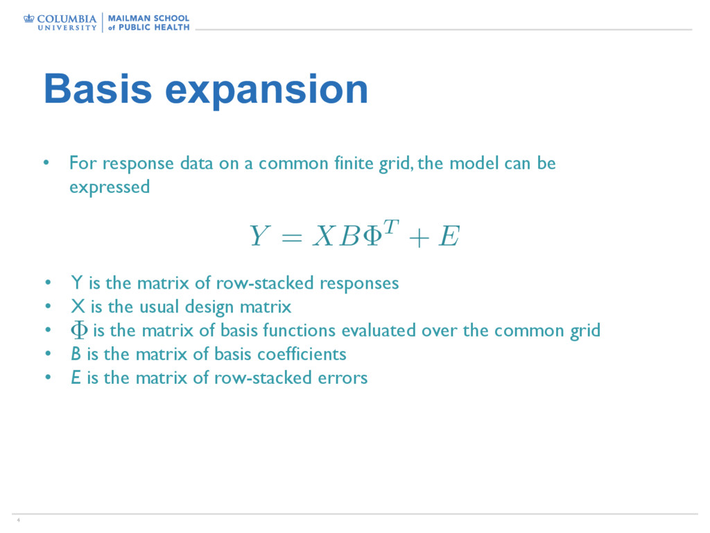
4. 4 Basis expansion • For response data on a common finite grid, the model can be expressed • Y is the matrix of row-stacked responses • X is the usual design matrix • is the matrix of basis functions evaluated over the common grid • B is the matrix of basis coefficients • E is the matrix of row-stacked errors Y = XB T + E
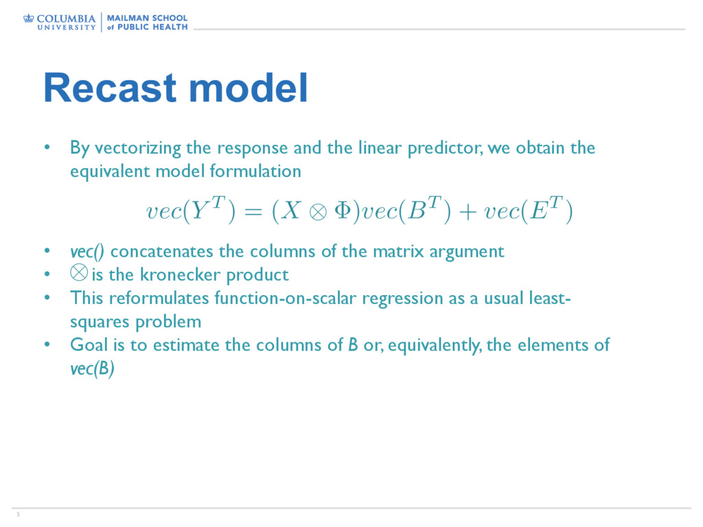
5. 5 Recast model • By vectorizing the response and the linear predictor, we obtain the equivalent model formulation vec(Y T ) = (X ⌦ )vec(BT ) + vec(ET ) • vec() concatenates the columns of the matrix argument • is the kronecker product • This reformulates function-on-scalar regression as a usual least- squares problem • Goal is to estimate the columns of B or, equivalently, the elements of vec(B) ⌦
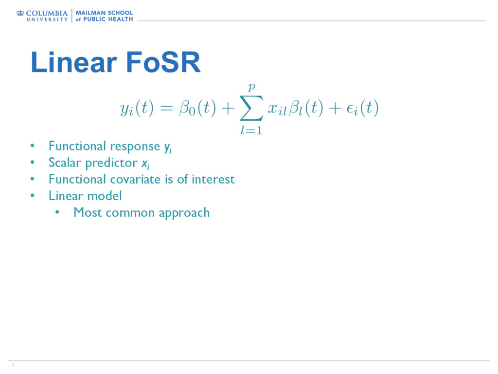
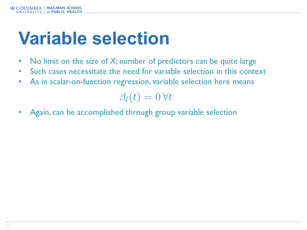
6. 6 Variable selection • No limit on the size of X; number of predictors can be quite large • Such cases necessitate the need for variable selection in this context • As in scalar-on-function regression, variable selection here means • Again, can be accomplished through group variable selection l(t) = 0 8t
7. 7 Scaling predictors • Much easier in this setting – usual scaling applies
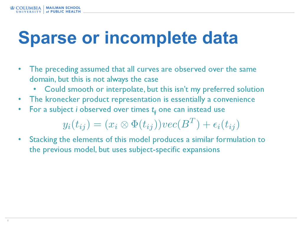
8. 8 Sparse or incomplete data • The preceding assumed that all curves are observed over the same domain, but this is not always the case • Could smooth or interpolate, but this isn’t my preferred solution • The kronecker product representation is essentially a convenience • For a subject i observed over times tij one can instead use • Stacking the elements of this model produces a similar formulation to the previous model, but uses subject-specific expansions yi( tij) = ( xi ⌦ ( tij)) vec ( B T ) + ✏i( tij)
9. 9 Correlated errors • Errors are correlated within a subject, but variable selection methods assume independent errors • Three approaches: • Ignore this issue • Use GLS in place of OLS by “pre-whitening” the left and right side of the matrix formulation of the model: • I.e. define where is the error covariance matrix, and similarly modify the RHS • Jointly model the coefficient vector and the residual covariance • Easiest in a Bayesian setting ✏i(t) ⌃ = LLT Y ⇤ = Y (L 1)T
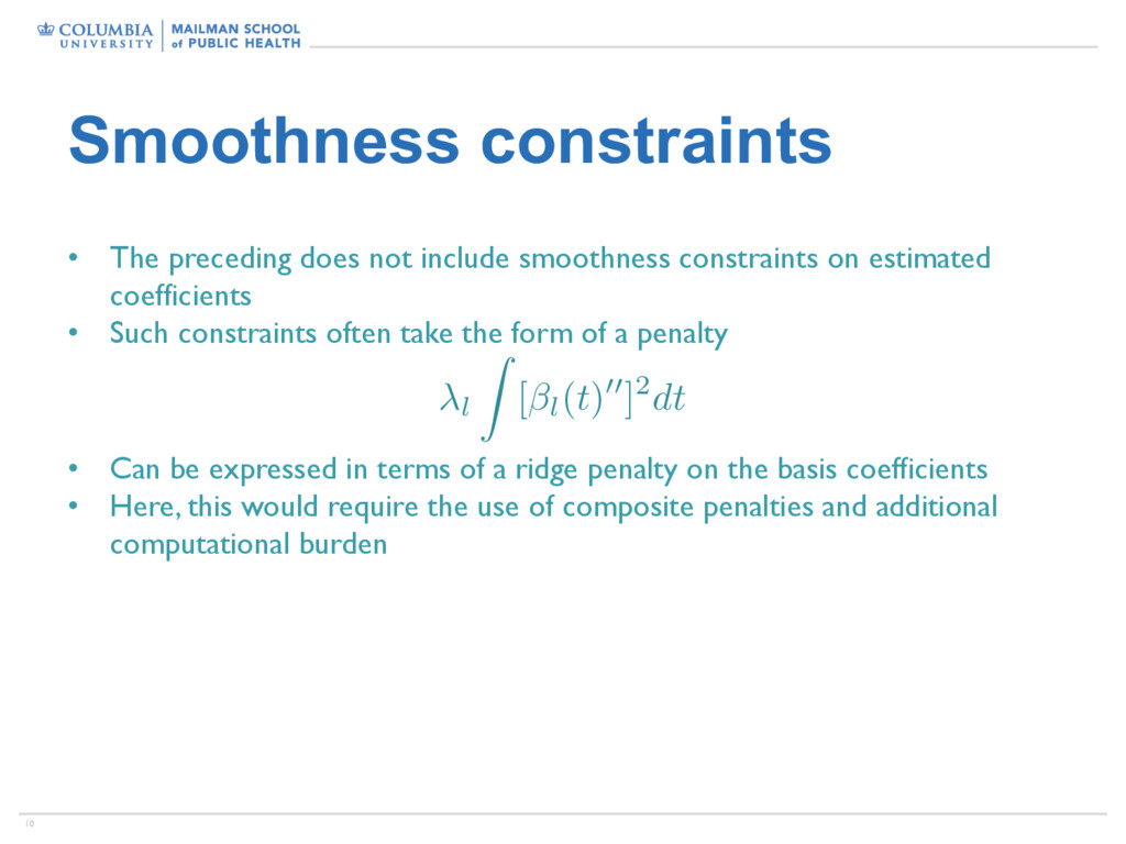
10. 10 Smoothness constraints • The preceding does not include smoothness constraints on estimated coefficients • Such constraints often take the form of a penalty l Z [ l(t)00]2dt • Can be expressed in terms of a ridge penalty on the basis coefficients • Here, this would require the use of composite penalties and additional computational burden
11. 11 Key references • Wang, Chen, and Li, (2007). Group SCAD regression analysis for microarray time course gene expression data. Bioinformatics. • Chen, Goldsmith, and Ogden (2016). Variable Selection in Function-on- Scalar Regression. Stat • Barber, Reimherr, and Schill (Submitted). The Function-on-Scalar LASSO with Applications to Longitudinal GWAS. • Parodi and Reimherr (Submitted). FLAME: Simultaneous variable selection and smoothing for high-dimensional function-on-scalar regression.
12. 12 Switch to code