misfitdislocations-another-method

heterointerfaces,interfaces,misfit dislocations,modeling

Transcript

1. Characterizing misfit dislocations at interfaces: Yet Another Method! Kedarnath Kolluri, M. J. Demkowicz Financial Support: Center for Materials at Irradiation and Mechanical Extremes (CMIME) at LANL, an Energy Frontier Research Center (EFRC) funded by U.S. Department of Energy, Office of Science, Office of Basic Energy Sciences Acknowledgments: A. Kashinath, A. Vattré, B. Uberuaga, X.-Y. Liu, A. Caro, and A. Misra
2. Classifying interfaces: Coherent, semi-coherent, and incoherent boundaries simplified side view • Lower and upper grains are in “perfect” alignment always
3. 1 4 8 12 1 4 8 13 • Lines of atoms are aligned perfectly only periodically Classifying interfaces: Coherent, semi-coherent, and incoherent boundaries simplified side view
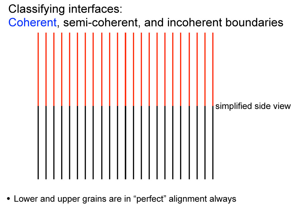
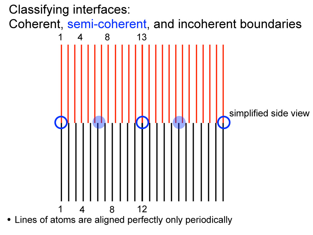
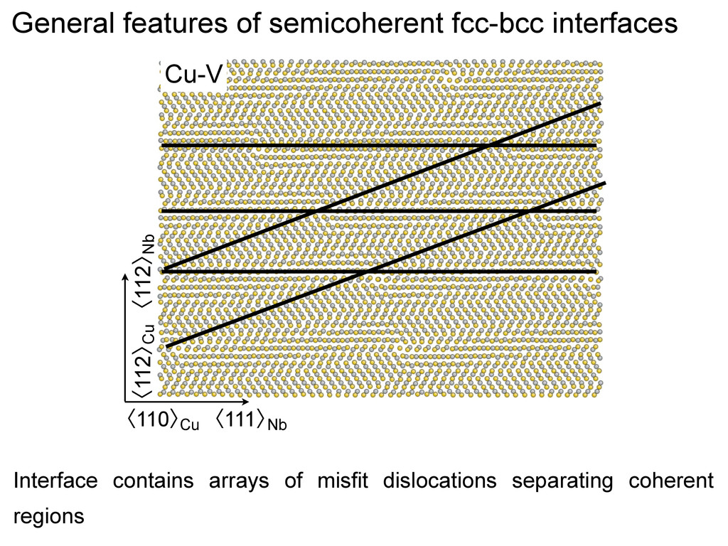
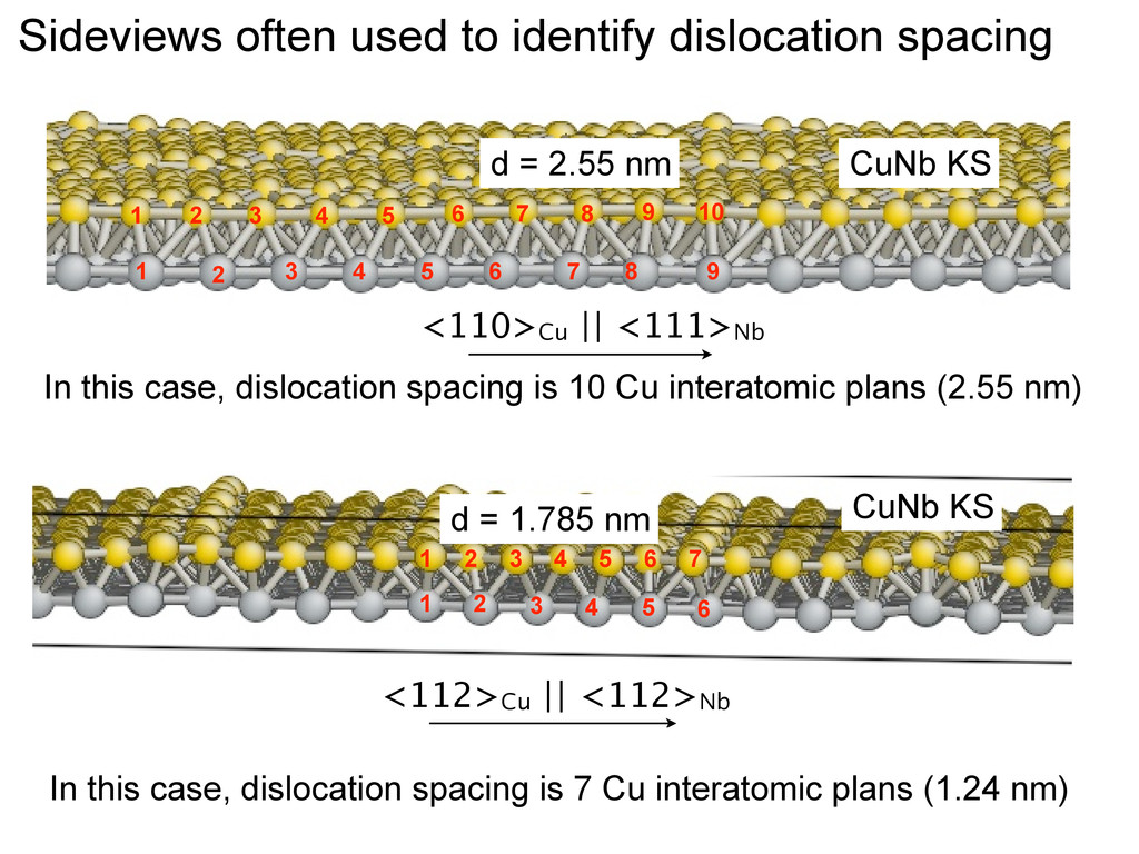
4. Coherent, semi-coherent, and incoherent boundaries • Atomic interactions generally reduce the “bad” patch • Coherent region experiences strain emanated by the “bad” patch • Interface with well separated “bad” patches may be described within the same theory as that of dislocations: misfit dislocations simplified side view Semi-coherent interfaces (2D defects) can be represented as arrays of dislocations (1D defects)
5. Line defects in metals: Edge dislocation Defects in Crystals, H. Foell. http://www.tf.uni-kiel.de/matwis/amat/def_en
6. Defects in Crystals, H. Foell. http://www.tf.uni-kiel.de/matwis/amat/def_en Line defects in metals: Screw dislocation
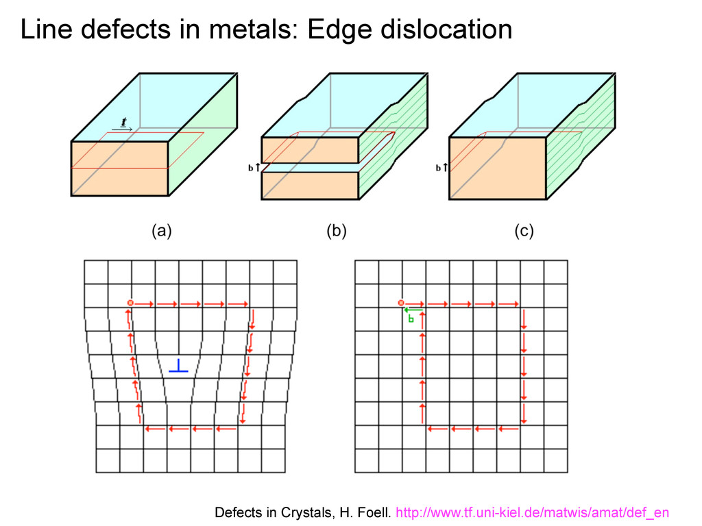
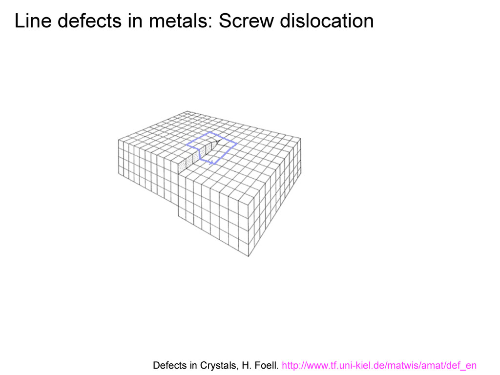
7. Dislocations screw dislocation edge dislocation • Dislocation • has a core (linear elasticity is inapplicable) • has a line vector (1-d defects) • described by a vector that displaces atoms when it moves Defects in Crystals, H. Foell. http://www.tf.uni-kiel.de/matwis/amat/def_en
8. Semi-coherent interfaces Semi-coherent interfaces (2D defects) can be represented as arrays of dislocations (1D defects)
9. General features of semicoherent fcc-bcc interfaces Cu-V ʪ110ʫ Cu ʪ111ʫ Nb ʪ112ʫ Cu ʪ112ʫ Nb An example of a semicoherent interface
10. View of the Interface
11. View of the Interface
12. View of the Interface
13. View of the Interface
14. View of the Interface
15. View of the Interface
16. General features of semicoherent fcc-bcc interfaces Cu-V ʪ110ʫ Cu ʪ111ʫ Nb ʪ112ʫ Cu ʪ112ʫ Nb An example of a fcc-bcc semicoherent interface Patterns corresponding to periodic “good” and “bad” regions
17. General features of semicoherent fcc-bcc interfaces Cu-V ʪ110ʫ Cu ʪ111ʫ Nb ʪ112ʫ Cu ʪ112ʫ Nb Interface contains arrays of misfit dislocations separating coherent regions
18. General features of semicoherent fcc-bcc interfaces ʪ110ʫ Cu ʪ111ʫ Nb ʪ112ʫ Cu ʪ112ʫ Nb Cu-Nb Cu-V Interface contains arrays of misfit dislocations separating coherent regions
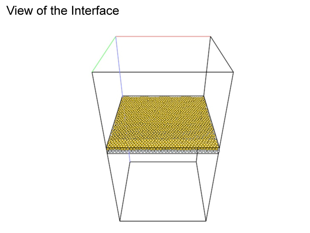
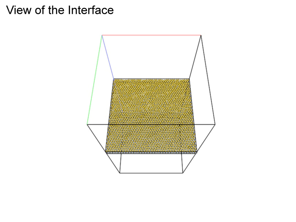
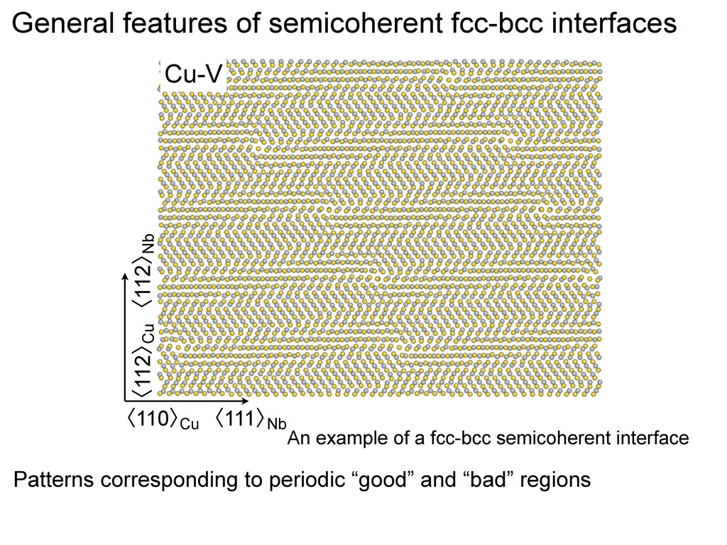
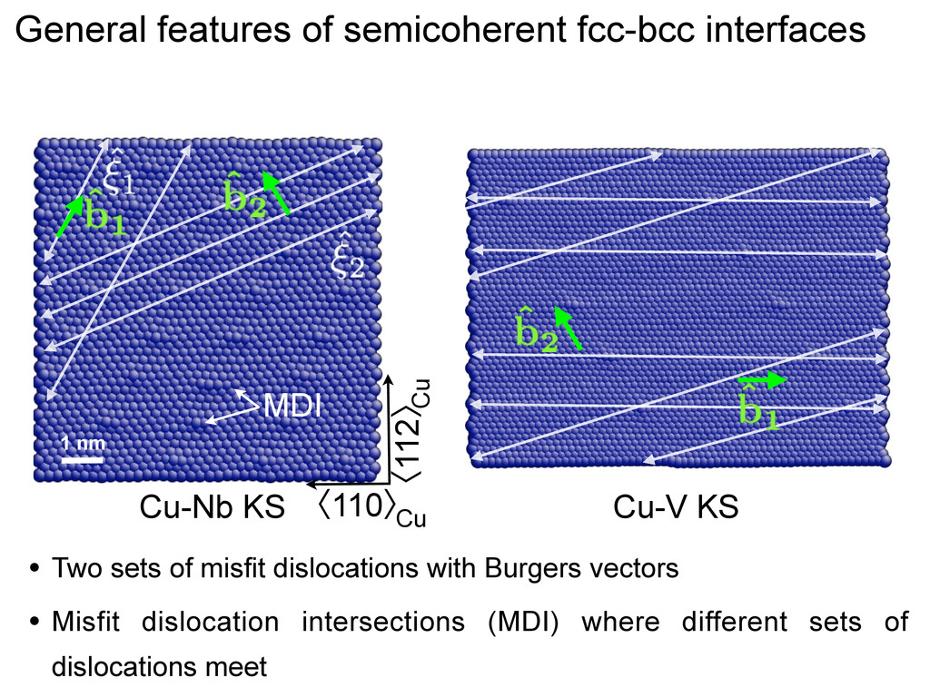
19. Cu-Nb KS Cu-V KS ʪ110ʫ Cu ʪ112ʫ Cu 1 nm MDI • Two sets of misfit dislocations with Burgers vectors • Misfit dislocation intersections (MDI) where different sets of dislocations meet General features of semicoherent fcc-bcc interfaces
20. Sideviews often used to identify dislocation spacing In this case, dislocation spacing is 10 Cu interatomic plans (2.55 nm) <112>Cu || <112>Nb 1 2 3 4 5 6 7 1 2 3 4 5 6 <110>Cu || <111>Nb 1 2 3 4 5 6 7 8 9 10 1 2 3 4 5 6 7 8 9 d = 2.55 nm CuNb KS In this case, dislocation spacing is 7 Cu interatomic plans (1.24 nm) <112>Cu || <112>Nb 1 2 3 4 5 6 7 1 2 3 4 5 6 <110>Cu || <111>Nb 1 2 3 4 5 6 7 8 9 10 1 2 3 4 5 6 7 8 9 d = 1.785 nm CuNb KS
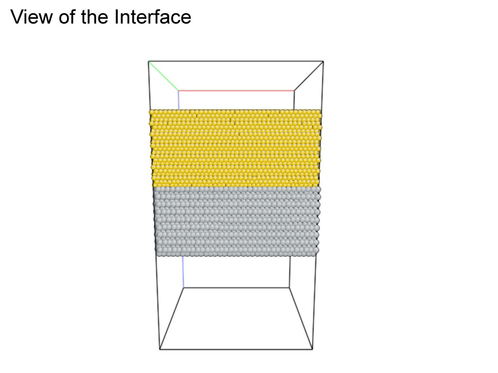
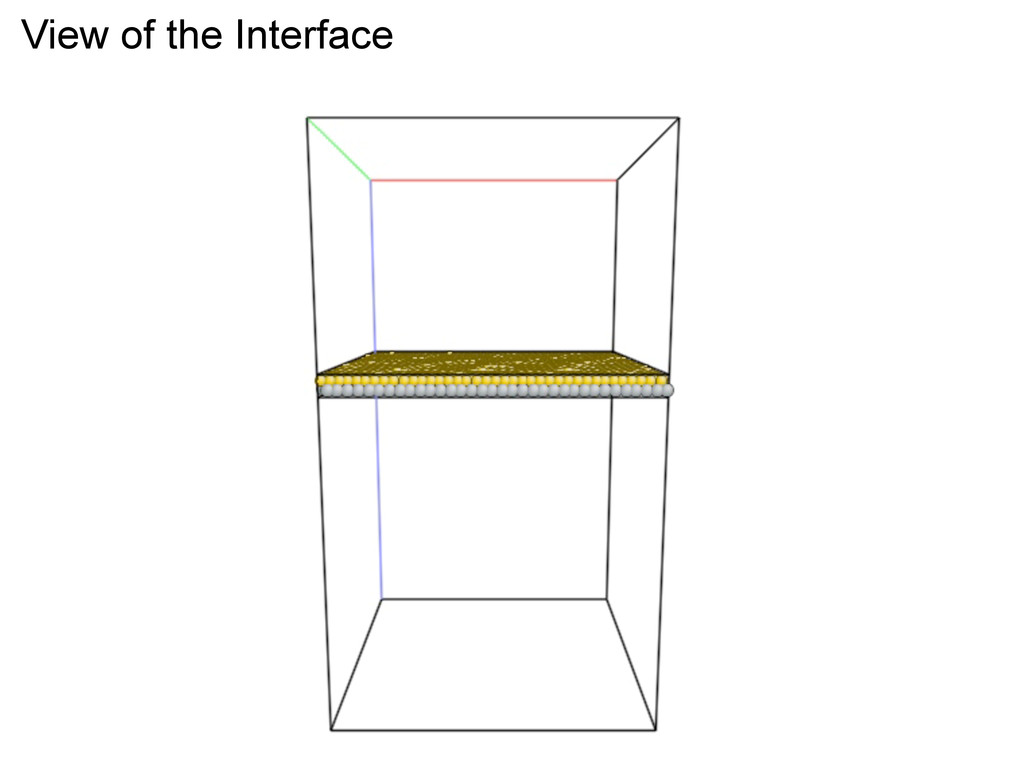
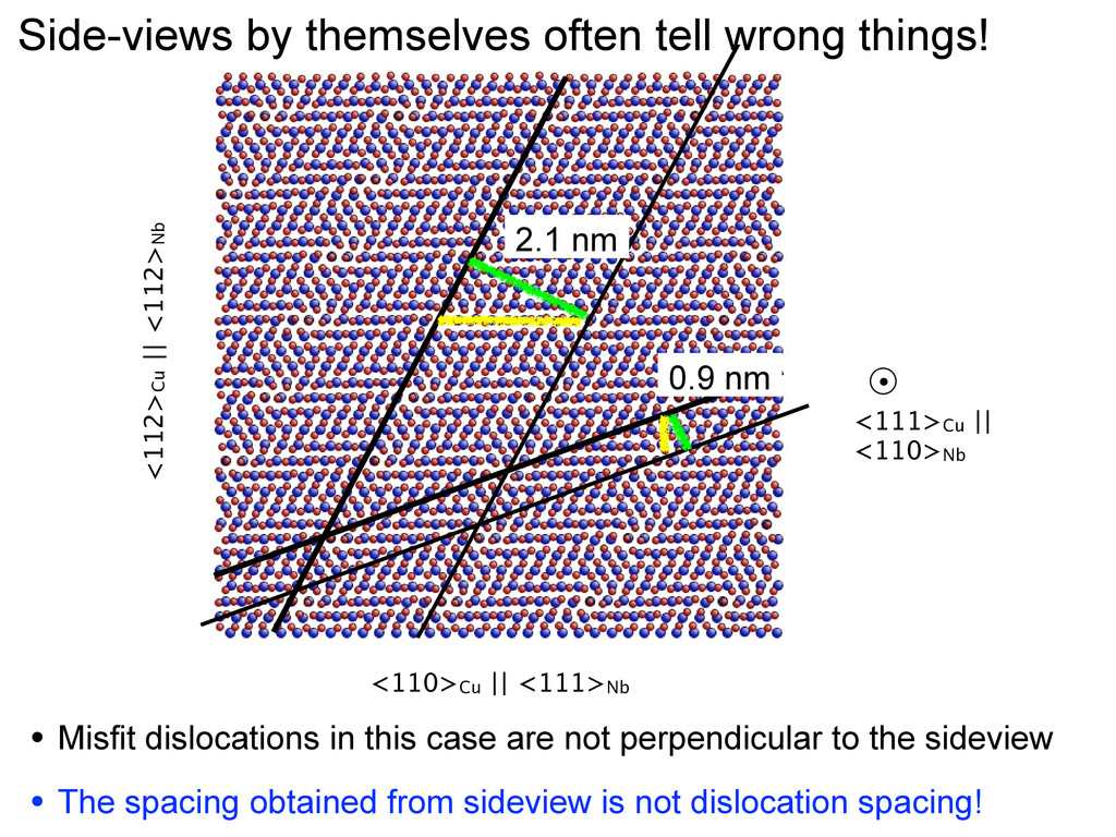
21. 12 <112>Cu || <112>Nb <110>Cu || <111>Nb <111>Cu || <110>Nb 2.1 nm 0.9 nm Side-views by themselves often tell wrong things! • Misfit dislocations in this case are not perpendicular to the sideview • The spacing obtained from sideview is not dislocation spacing!
22. Yet another method for finding dislocations at fcc-bcc interfaces
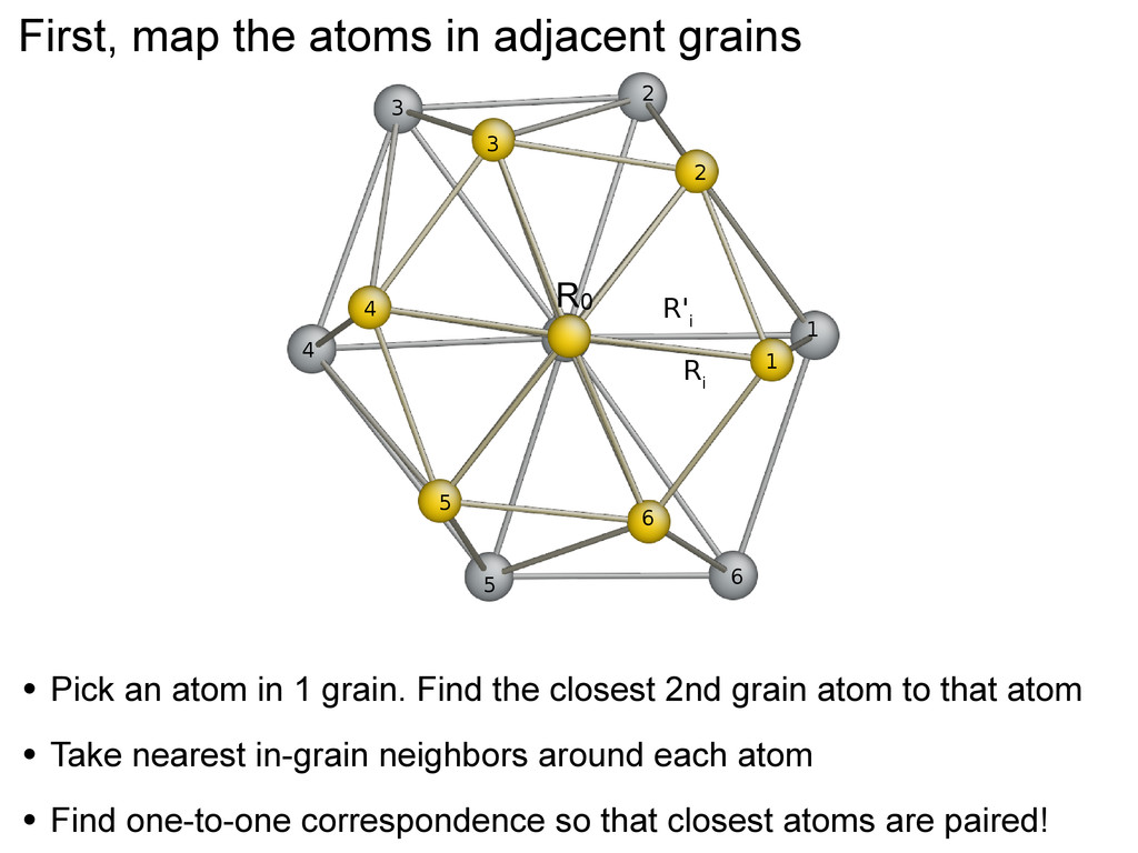
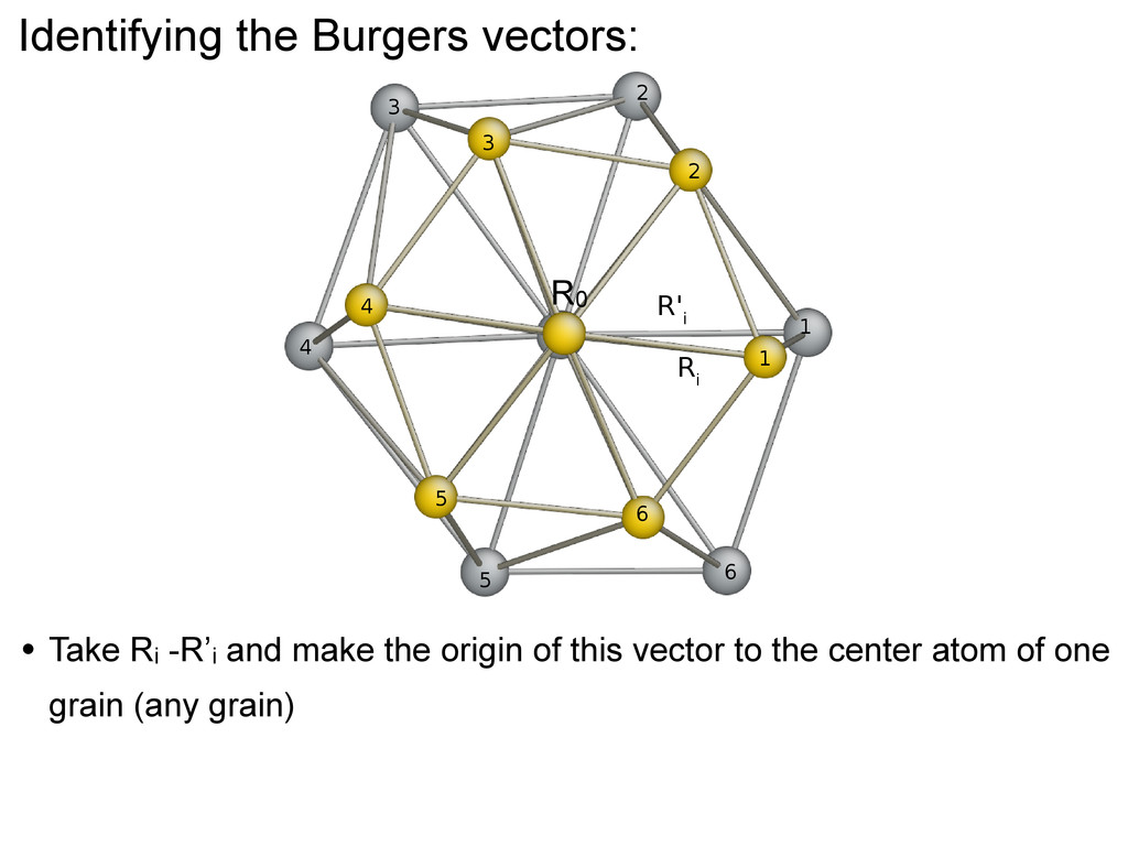
23. First, map the atoms in adjacent grains R i R' i Compute vectors R'i-Ri where the vectors are the lines joining the closest fcc and bcc atoms to their corresponding nearest neighbors 1 1 1 2 2 3 3 4 4 5 5 6 6 Cu-Fe NW R0 • Pick an atom in 1 grain. Find the closest 2nd grain atom to that atom • Take nearest in-grain neighbors around each atom • Find one-to-one correspondence so that closest atoms are paired!
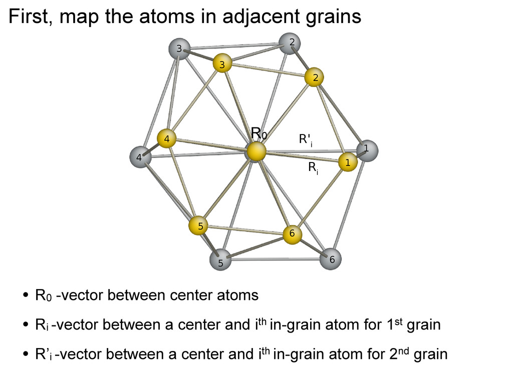
24. First, map the atoms in adjacent grains • R0 -vector between center atoms • Ri -vector between a center and ith in-grain atom for 1st grain • R’i -vector between a center and ith in-grain atom for 2nd grain R i R' i Compute vectors R'i-Ri where the vectors are the lines joining the closest fcc and bcc atoms to their corresponding nearest neighbors 1 1 1 2 2 3 3 4 4 5 5 6 6 Cu-Fe NW R0
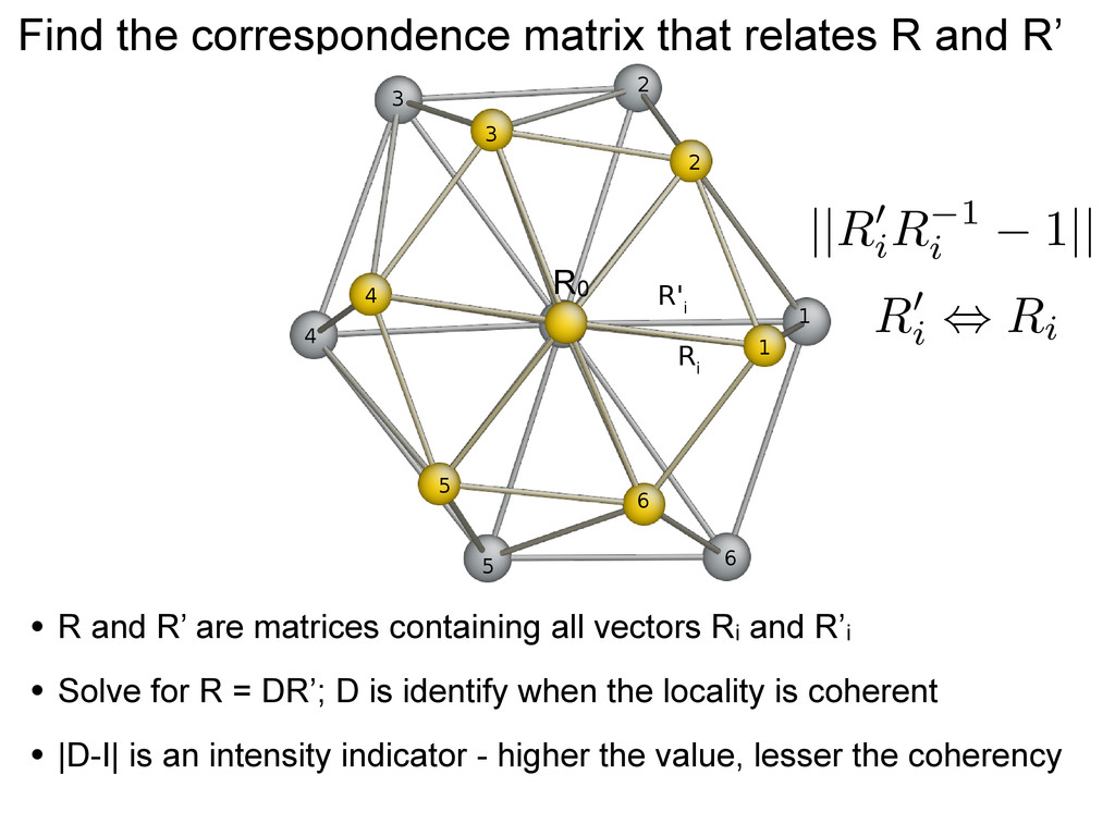
25. Find the correspondence matrix that relates R and R’ R i R' i Compute vectors R'i-Ri where the vectors are the lines joining the closest fcc and bcc atoms to their corresponding nearest neighbors 1 1 1 2 2 3 3 4 4 5 5 6 6 Cu-Fe NW R0 R0 i , Ri • R and R’ are matrices containing all vectors Ri and R’i • Solve for R = DR’; D is identify when the locality is coherent • |D-I| is an intensity indicator - higher the value, lesser the coherency ||R0 i R 1 i 1||
26. D=I for perfect system like the one here Adjacent planes of fcc (Cu) 1 2 3 4 5 6 C 1 2 3 4 5 6 C
27. An example result 0.3 0.35 0.4 0.45 0.5 0.55 0.6 0.3 0.35 0.4 0.45 0.5 0.55 0.6 fcc<112> fcc<110> NW Cu-Fe 0.05 0.1 0.15 0.2 0.25 0.3 CuFe NW |D-I| Cu<110> Cu<112> • Identifies dislocations well! • But do information about the characteristics of the dislocation!
28. Structure of interfaces: Misfit dislocations • A general method to identify dislocation line and Burgers vectors • Assumption: A coherent patch exists at the interface • Advantage: Reference structure not required • Limitations: Dislocation core thickness cannot be determined (yet)
29. Identifying the Burgers vectors: • Take Ri -R’i and make the origin of this vector to the center atom of one grain (any grain) R i R' i Compute vectors R'i-Ri where the vectors are the lines joining the closest fcc and bcc atoms to their corresponding nearest neighbors 1 1 1 2 2 3 3 4 4 5 5 6 6 Cu-Fe NW R0
30. The computed vectors are plotted. The vectors all originate at the location of the center atom shown in slide 1 fcc<110> fcc<112> First, take Ri-R’i and place it about the center atom CuFe NW
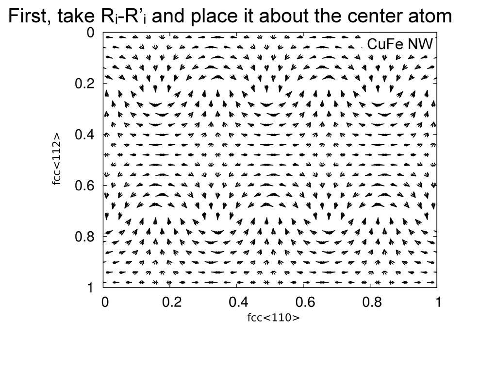
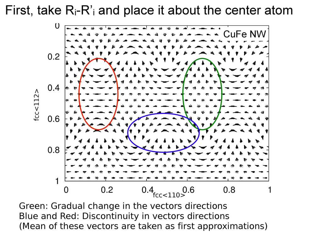
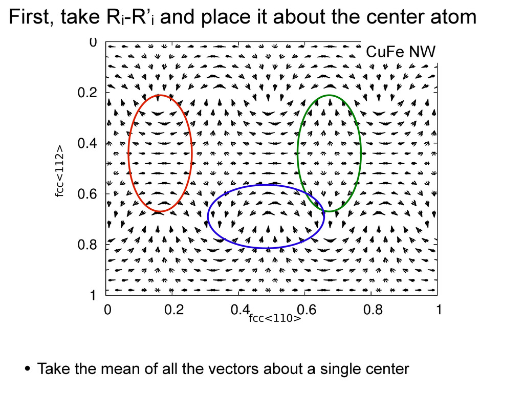
31. Green: Gradual change in the vectors directions Blue and Red: Discontinuity in vectors directions (Mean of these vectors are taken as first approximations) fcc<110> fcc<112> First, take Ri-R’i and place it about the center atom CuFe NW
32. Green: Gradual change in the vectors directions Blue and Red: Discontinuity in vectors directions (Mean of these vectors are taken as first approximations) fcc<110> fcc<112> First, take Ri-R’i and place it about the center atom • Take the mean of all the vectors about a single center CuFe NW
33. Reduce dimensions by simple average of vectors • Take average of local deviations (differentiating) of the vectors CuFe NW
34. The directions give the Burgers vectors Reduce dimensions by simple average of vectors CuFe NW
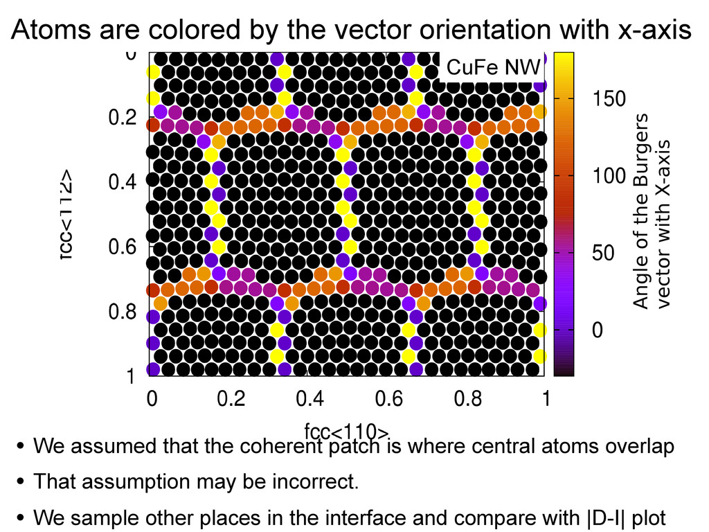
35. Atoms are colored by the vector orientation with x-axis Angle of the Burgers vector with X-axis Yellow and light blue: BV is 180 or 0 degrees with +x-axis Purple : BV is 60 degrees with +x-axis Orange : BV is 120 degrees with +x-axis CuFe NW
36. Atoms are colored by the vector orientation with x-axis Angle of the Burgers vector with X-axis Yellow and light blue: BV is 180 or 0 degrees with +x-axis Purple : BV is 60 degrees with +x-axis Orange : BV is 120 degrees with +x-axis • We assumed that the coherent patch is where central atoms overlap • That assumption may be incorrect. • We sample other places in the interface and compare with |D-I| plot CuFe NW
37. .3 35 .4 45 .5 55 .6 0.3 0.35 0.4 0.45 0.5 0.55 0.6 fcc<110> NW Cu-Fe 0 50 100 150 0.3 0.35 0.4 0.45 0.5 0.55 0.6 0.3 0.35 0.4 0.45 0.5 0.55 0.6 fcc<112> fcc<110> NW Cu-Fe 0 50 100 150 0.3 0.35 0.4 0.45 0.5 0.55 0.6 0.3 0.35 0.4 0.45 0.5 0.55 0.6 fcc<112> fcc<110> NW 0 5 1 1 Comparing various possible coherent patchs with |D-I| 0.3 0.35 0.4 0.45 0.5 0.55 0.6 fcc<112> NW Cu-Fe 0.05 0.1 0.15 0.2 0.25 0.3 CuFe NW |D-I| map
38. K. Kolluri, and M. J. Demkowicz, unpublished Example results and limitations! • A general method to identify dislocation line and Burgers vectors • Assumption: A coherent patch exists at the interface • Advantage: Reference structure not required • Limitations: Dislocation core thickness cannot be determined (yet) .2 0.4 0.6 0.8 1 0.15 0.2 0.25 0.3 0.35 0.4 0.45 0.5 0 0 0.2 0.4 0.6 0.8 1 0 50 100 150 0 0.2 0.4 0.6 0.8 1 0 0.4 0.6 0.8 1 0 50 100 150 0 0.2 0.4 0.6 0.8 1 0 0.2 0.4 0.6 0.8 1 0.06 0.08 0.1 0.12 0.14 0.16 0.18 0.2 0.22 0.24 0.26 0.28 Angle with -ve x axis 0 50 100 150 Angle with -ve x-axis