ROMS turbulence parameter comparisons with field data

Poster presented at the Physics of Estuaries and Coastal Seas (PECS) conference in New York City, August 2012.

Transcript

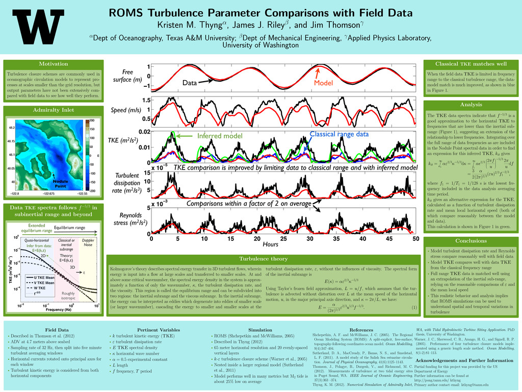
1. ROMS Turbulence Parameter Comparisons with Field Data Kristen M. Thyngα, James J. Rileyβ, and Jim Thomsonγ αDept of Oceanography, Texas A&M University; βDept of Mechanical Engineering, γApplied Physics Laboratory, University of Washington Motivation Turbulence closure schemes are commonly used in oceanographic circulation models to represent pro- cesses at scales smaller than the grid resolution, but output parameters have not been extensively com- pared with field data to see how well they perform. Admiralty Inlet Nodule Point Data TKE spectra follows f−5/3 in subinertial range and beyond 10−2 10−1 100 101 10−4 10−3 10−2 10−1 100 Frequency (Hz) TKE (m2/s2 Hz−1) U TKE Mean V TKE Mean W TKE f−5/3 Classical or inertial subrange Equilibrium range 3D Theory: E=E(k,ε) Quasi-horizontal Roughly isotropic ε 2D Doppler Noise Extended equilibrium range Infer from data: E=E(k,ε) −1 0 1 Free Surface (m) 0.5 1 1.5 Speed (m/s) 0 0.01 0.02 TKE (m2/s2) 5 10 15 x 10−5 Turbulent Dissipation Rate (m2/s3) 0 5 10 15 20 25 30 35 40 45 50 0 5 x 10−3 Reynolds Stress (m2/s2) Hours into comparison Free surface (m) Speed (m/s) TKE (m2/s2) Turbulent dissipation rate (m2/s3) Reynolds stress (m2/s2) Data Model Classical range data Inferred model Hours Comparisons within a factor of 2 on average TKE comparison is improved by limiting data to classical range and with inferred model Turbulence theory Kolmogorov’s theory describes spectral energy transfer in 3D turbulent flows, wherein energy is input into a flow at large scales and transferred to smaller scales. At and above some critical wavenumber, the spectral energy density in the system is approx- imately a function of only the wavenumber, κ, the turbulent dissipation rate, and the viscosity. This region is called the equilibrium range and can be subdivided into two regions: the inertial subrange and the viscous subrange. In the inertial subrange, the energy can be interpreted as eddies which degenerate into eddies of smaller scale (or larger wavenumber), cascading the energy to smaller and smaller scales at the turbulent dissipation rate, ε, without the influences of viscosity. The spectral form of the inertial subrange is E(κ) = αε2/3κ−5/3 Using Taylor’s frozen field approximation, L = u/f, which assumes that the tur- bulence is advected without distortion over L at the mean speed of the horizontal motion, u, in the major principal axis direction, and κ = 2π/L, we have: E = α (2π)5/3 ε2/3u5/3f−5/3. (1) Classical TKE matches well When the field data TKE is limited in frequency range to the classical turbulence range, the data- model match is much improved, as shown in blue in Figure 1. Analysis The TKE data spectra indicate that f−5/3 is a good approximation to the horizontal TKE to frequencies that are lower than the inertial sub- range (Figure 1), suggesting an extension of the relationship to lower frequencies. Integrating over the full range of data frequencies as are included in the Nodule Point spectral data in order to find an expression for this inferred TKE, kit gives kit = ∞ κ1 αε2/3κ−5/3dκ = ∞ f1 α 2/3        2πf u        −5/3 2π u df = 3 2 α (2π)2/3 (εu)2/3f−2/3 1 , where f1 = 1/T1 = 1/128 s is the lowest fre- quency included in the data analysis averaging time period. kit gives an alternative expression for the TKE, calculated as a function of turbulent dissipation rate and mean local horizontal speed (both of which compare reasonably between the model and data). This calculation is shown in Figure 1 in green. Conclusions • Model turbulent dissipation rate and Reynolds stress compare reasonably well with field data • Model TKE compares well with data TKE from the classical frequency range • Full range TKE data is matched well using an extrapolation of the inertial sub-range, relying on the reasonable comparisons of ε and the mean local speed • This realistic behavior and analysis implies that ROMS simulations can be used to understand spatial and temporal variations in turbulence Field Data • Described in Thomson et al. (2012) • ADV at 4.7 meters above seabed • Sampling rate of 32 Hz, then split into five minute turbulent averaging windows • Horizontal currents rotated onto principal axes for each window • Turbulent kinetic energy is considered from both horizontal components Pertinent Variables • k turbulent kinetic energy (TKE) • ε turbulent dissipation rate • E TKE spectral density • κ horizontal wave number • α = 0.5 experimental constant • L length • f frequency, T period Simulation • ROMS (Shchepetkin and McWilliams, 2005) • Described in Thyng (2012) • 65 meter horizontal resolution and 20 evenly-spaced vertical layers • k-ε turbulence closure scheme (Warner et al., 2005) • Nested inside a larger regional model (Sutherland et al., 2011) • Model performs well in many metrics but M2 tide is about 25% low on average References Shchepetkin, A. F. and McWilliams, J. C. (2005). The Regional Ocean Modeling System (ROMS): A split-explicit, free-surface, topography-following coordinates ocean model. Ocean Modelling, 9(4):347–404. Sutherland, D. A., MacCready, P., Banas, N. S., and Smedstad, L. F. (2011). A model study of the Salish Sea estuarine circula- tion. Journal of Physical Oceanography, 41(6):1125–1143. Thomson, J., Polagye, B., Durgesh, V., and Richmond, M. C. (2012). Measurements of turbulence at two tidal energy sites in Puget Sound, WA. IEEE Journal of Oceanic Engineering, 37(3):363 –374. Thyng, K. M. (2012). Numerical Simulation of Admiralty Inlet, WA, with Tidal Hydrokinetic Turbine Siting Application. PhD thesis, University of Washington. Warner, J. C., Sherwood, C. R., Arango, H. G., and Signell, R. P. (2005). Performance of four turbulence closure models imple- mented using a generic length scale method. Ocean Modelling, 8(1-2):81–113. Acknowledgements and Further Information Partial funding for this project was provided by the US Department of Energy Further information can be found at http://pong.tamu.edu/ kthyng Primary author contact email: kthyng@tamu.edu