FALSEだと等分散性を仮定し ない(Welchの方法) > t.test(seiseki[, 2], seiseki[, 3], paired = TRUE, var.equal = FALSE) Paired t-test data: seiseki[, 2] and seiseki[, 3] t = 2.1301, df = 49, p-value = 0.03821 alternative hypothesis: true difference in means is not equal to 0 95 percent confidence interval: 0.1980557 6.8019443 sample estimates: mean of the differences 3.5
rank sum test with continuity correction data: seiseki[, 2] and seiseki[, 3] W = 1369.5, p-value = 0.4118 alternative hypothesis: true location shift is not equal to 0
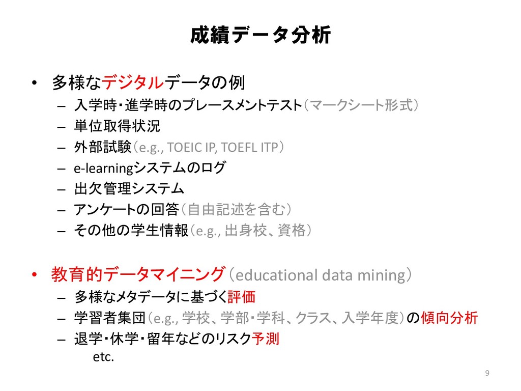
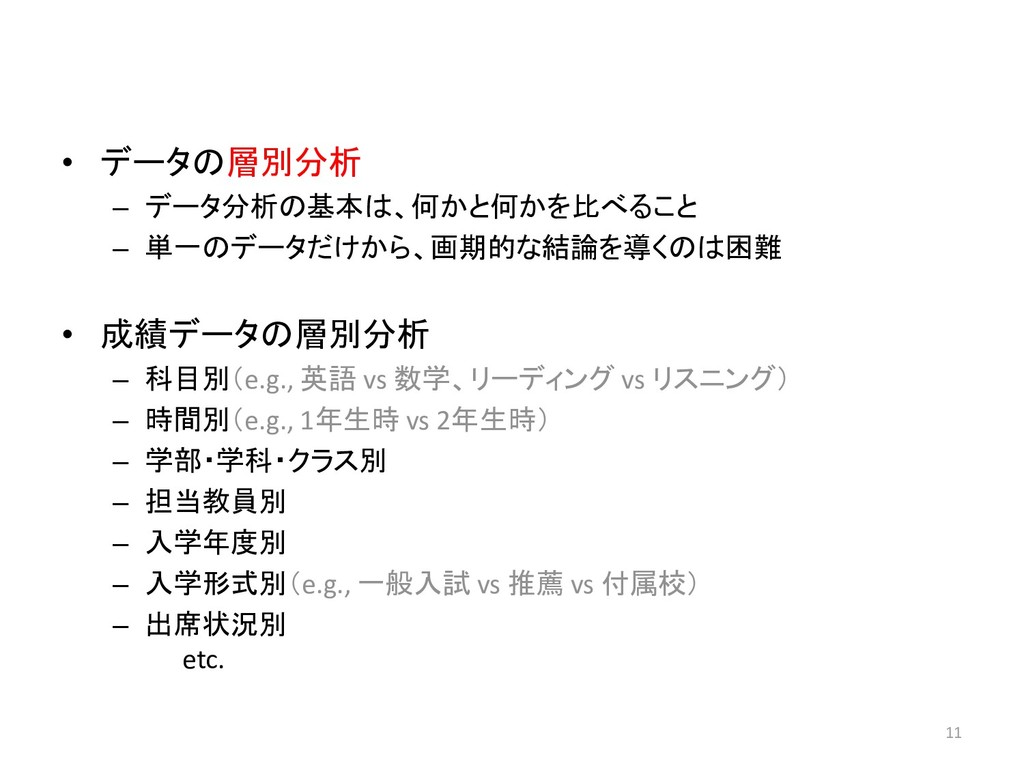
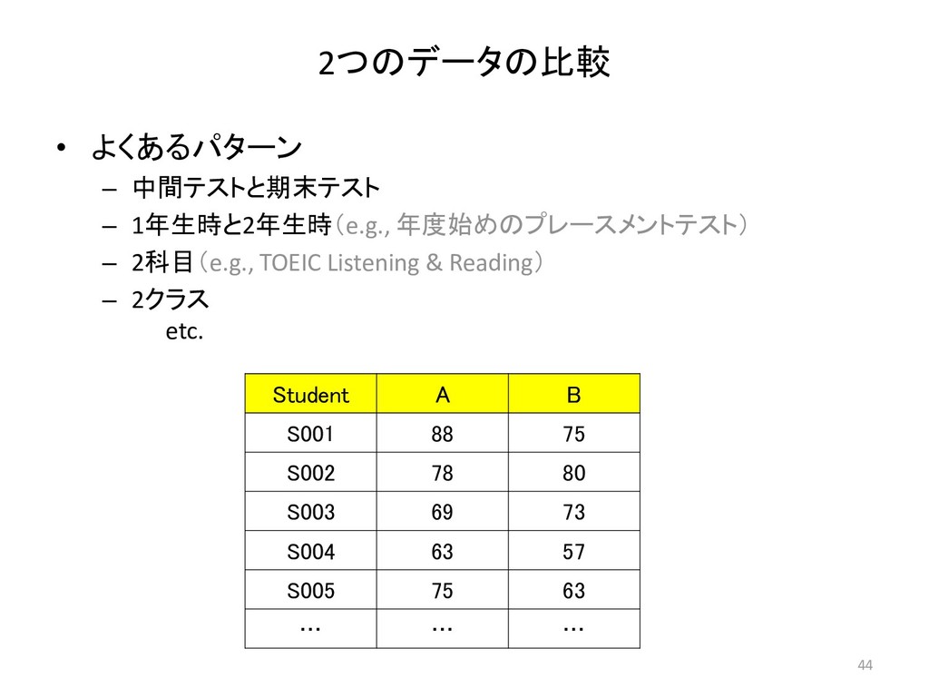
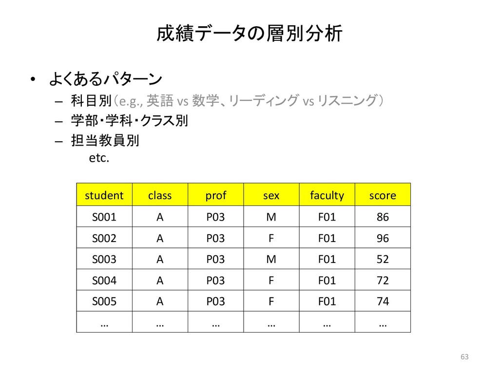
– 学部・学科・クラス別 – 担当教員別 etc. 63 student class prof sex faculty score S001 A P03 M F01 86 S002 A P03 F F01 96 S003 A P03 M F01 52 S004 A P03 F F01 72 S005 A P03 F F01 74 … … … … … …
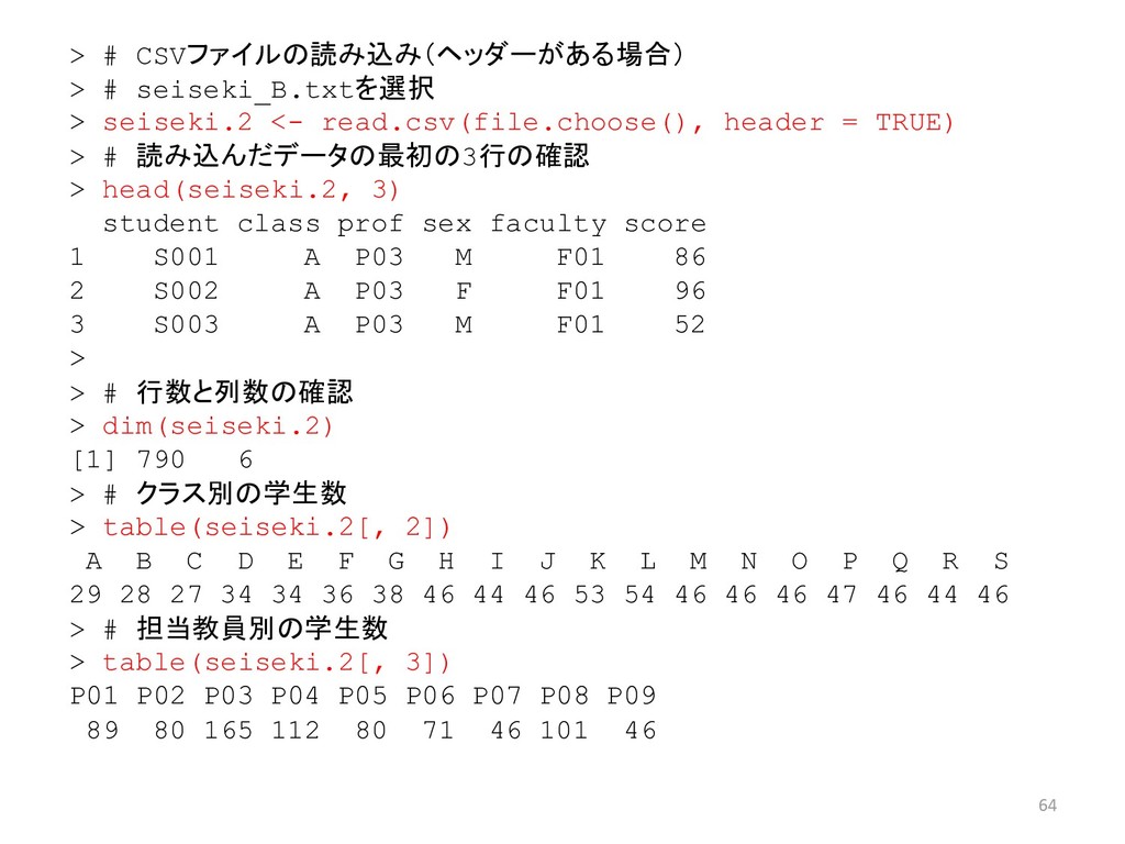
read.csv(file.choose(), header = TRUE) > # 読み込んだデータの最初の3行の確認 > head(seiseki.2, 3) student class prof sex faculty score 1 S001 A P03 M F01 86 2 S002 A P03 F F01 96 3 S003 A P03 M F01 52 > > # 行数と列数の確認 > dim(seiseki.2) [1] 790 6 > # クラス別の学生数 > table(seiseki.2[, 2]) A B C D E F G H I J K L M N O P Q R S 29 28 27 34 34 36 38 46 44 46 53 54 46 46 46 47 46 44 46 > # 担当教員別の学生数 > table(seiseki.2[, 3]) P01 P02 P03 P04 P05 P06 P07 P08 P09 89 80 165 112 80 71 46 101 46
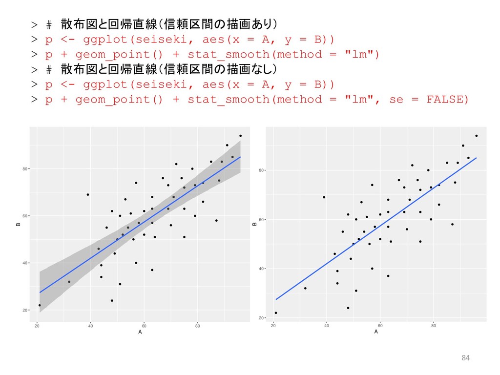
A, y = B)) > p + geom_point() + stat_smooth(method = "lm") > # 散布図と回帰直線(信頼区間の描画なし) > p <- ggplot(seiseki, aes(x = A, y = B)) > p + geom_point() + stat_smooth(method = "lm", se = FALSE) 20 40 60 80 20 40 60 80 A B 20 40 60 80 20 40 60 80 A B
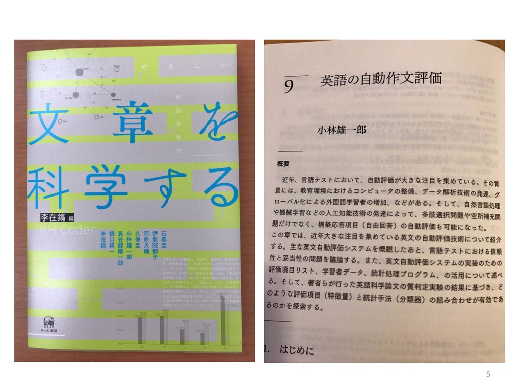
![• 単著 – 『Rによるやさしいテキストマイニング』(オーム社、2017) – 『Rによるやさしいテキストマイニング[機械学習編]』(オーム社、2017) – 『仕事に使えるクチコミ分析―テキストマイニングと統計学をマーケティ ングに活用する』(技術評論社、2017) –](https://files.speakerdeck.com/presentations/23dd3431d8b14a83ae49849b6ce92944/slide_5.jpg)
![概要 1. [講義] 成績データ分析 2. [講義] Rによるデータ分析 3. [実習] Rの基本](https://files.speakerdeck.com/presentations/23dd3431d8b14a83ae49849b6ce92944/slide_6.jpg)
![概要 1. [講義] 成績データ分析 2. [講義] Rによるデータ分析 3. [実習] Rの基本](https://files.speakerdeck.com/presentations/23dd3431d8b14a83ae49849b6ce92944/slide_7.jpg)
![概要 1. [講義] 成績データ分析 2. [講義] Rによるデータ分析 3. [実習] Rの基本](https://files.speakerdeck.com/presentations/23dd3431d8b14a83ae49849b6ce92944/slide_13.jpg)
![概要 1. [講義] 成績データ分析 2. [講義] Rによるデータ分析 3. [実習] Rの基本](https://files.speakerdeck.com/presentations/23dd3431d8b14a83ae49849b6ce92944/slide_16.jpg)
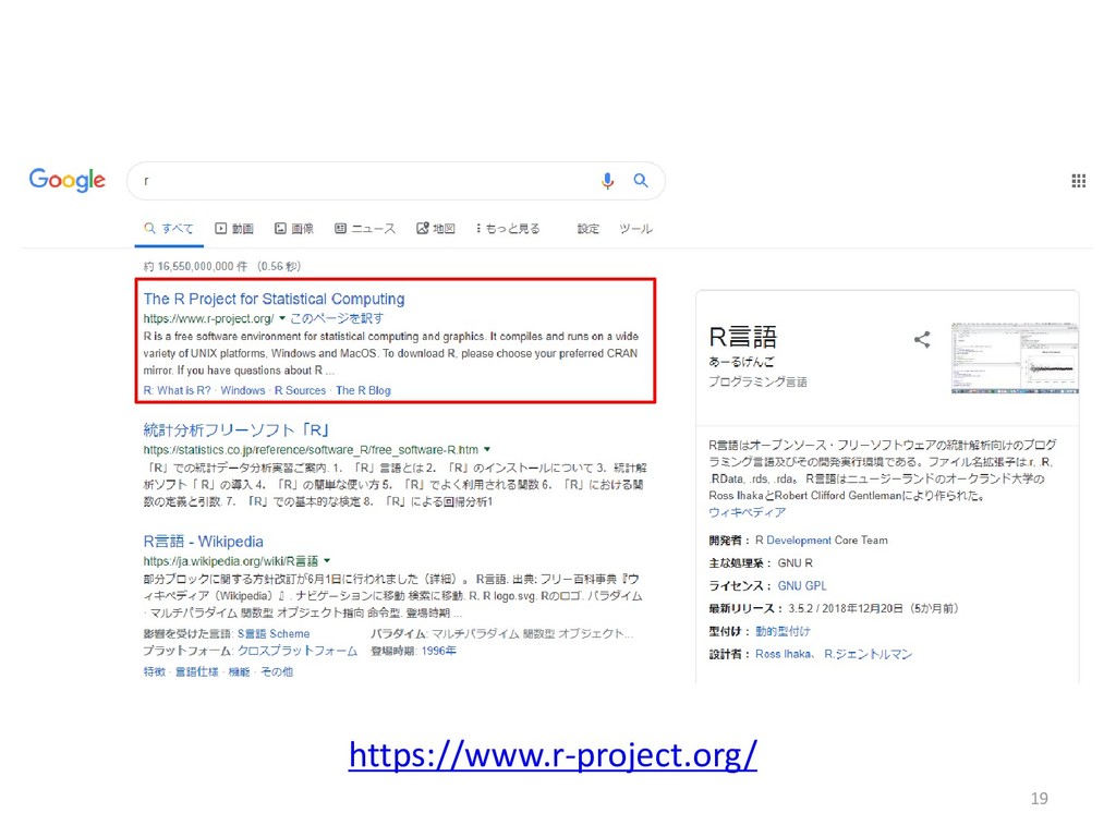
![21 [中略] Japanのいずれかのサイトへ(基本的には、どれでも同じ)](https://files.speakerdeck.com/presentations/23dd3431d8b14a83ae49849b6ce92944/slide_20.jpg)
![基本的なプログラミング 27 > # 入力練習 > 1 + 2 [1]](https://files.speakerdeck.com/presentations/23dd3431d8b14a83ae49849b6ce92944/slide_26.jpg)
![30 > # ベクトルを使った計算 > x * 2 [1] 2](https://files.speakerdeck.com/presentations/23dd3431d8b14a83ae49849b6ce92944/slide_29.jpg)
![32 > # 行列を使った計算 > matrix.2 + 1 [,1] [,2]](https://files.speakerdeck.com/presentations/23dd3431d8b14a83ae49849b6ce92944/slide_31.jpg)
![33 > # 行列の結合(列方向) > cbind(matrix.2, matrix.3) [,1] [,2] [,3]](https://files.speakerdeck.com/presentations/23dd3431d8b14a83ae49849b6ce92944/slide_32.jpg)
![34 > # 3列目の要素以外の全てを取り出し > matrix.2[, -3] [,1] [,2] [1,]](https://files.speakerdeck.com/presentations/23dd3431d8b14a83ae49849b6ce92944/slide_33.jpg)
![40 > # 行ごとの総和 > rowSums(matrix.4) [1] 6 15 24](https://files.speakerdeck.com/presentations/23dd3431d8b14a83ae49849b6ce92944/slide_39.jpg)
![41 > # 列ごとの要約統計量 > apply(matrix.4, 2, summary) [,1] [,2]](https://files.speakerdeck.com/presentations/23dd3431d8b14a83ae49849b6ce92944/slide_40.jpg)
![概要 1. [講義] 成績データ分析 2. [講義] Rによるデータ分析 3. [実習] Rの基本](https://files.speakerdeck.com/presentations/23dd3431d8b14a83ae49849b6ce92944/slide_42.jpg)
![48 > # ヒストグラムによるTest Aの可視化 > hist(seiseki[, 2]) > #](https://files.speakerdeck.com/presentations/23dd3431d8b14a83ae49849b6ce92944/slide_47.jpg)
![49 > # 幹葉図による可視化 > stem(seiseki[, 2]) The decimal point](https://files.speakerdeck.com/presentations/23dd3431d8b14a83ae49849b6ce92944/slide_48.jpg)
![50 > # 箱ひげ図による可視化 > boxplot(seiseki[, 2]) > # range](https://files.speakerdeck.com/presentations/23dd3431d8b14a83ae49849b6ce92944/slide_49.jpg)
![55 > # 箱ひげ図にbeeswarmを重ね描き > boxplot(seiseki[, 2], range = 0,](https://files.speakerdeck.com/presentations/23dd3431d8b14a83ae49849b6ce92944/slide_54.jpg)
![57 > # Wilcoxonの順位和検定 > wilcox.test(seiseki[, 2], seiseki[, 3]) Wilcoxon](https://files.speakerdeck.com/presentations/23dd3431d8b14a83ae49849b6ce92944/slide_56.jpg)
![58 > # 散布図 > plot(seiseki[, 2], seiseki[, 3]) >](https://files.speakerdeck.com/presentations/23dd3431d8b14a83ae49849b6ce92944/slide_57.jpg)
![59 > # Pearsonの積率相関係数 > cor(seiseki[, 2], seiseki[, 3], method](https://files.speakerdeck.com/presentations/23dd3431d8b14a83ae49849b6ce92944/slide_58.jpg)
![61 > # 散布図に回帰直線を重ね描き > plot(seiseki[, 2], seiseki[, 3], pch](https://files.speakerdeck.com/presentations/23dd3431d8b14a83ae49849b6ce92944/slide_60.jpg)
![概要 1. [講義] 成績データ分析 2. [講義] Rによるデータ分析 3. [実習] Rの基本](https://files.speakerdeck.com/presentations/23dd3431d8b14a83ae49849b6ce92944/slide_61.jpg)
![65 > # 男女別の学生数 > table(seiseki.2[, 4]) F M 236](https://files.speakerdeck.com/presentations/23dd3431d8b14a83ae49849b6ce92944/slide_64.jpg)
![67 > # 層別の要約統計量 > # クラス別の要約統計量 > tapply(seiseki.2[, 6],](https://files.speakerdeck.com/presentations/23dd3431d8b14a83ae49849b6ce92944/slide_66.jpg)
![68 > # 層別の箱ひげ図 > # クラス別の箱ひげ図 > boxplot(seiseki.2[, 6]](https://files.speakerdeck.com/presentations/23dd3431d8b14a83ae49849b6ce92944/slide_67.jpg)
![69 > # 担当教員別の箱ひげ図 > boxplot(seiseki.2[, 6] ~ seiseki.2[, 3],](https://files.speakerdeck.com/presentations/23dd3431d8b14a83ae49849b6ce92944/slide_68.jpg)
![74 > # 一元配置分散分析(等分散性を仮定) > oneway.test(seiseki.2[, 6] ~ seiseki.2[, 2],](https://files.speakerdeck.com/presentations/23dd3431d8b14a83ae49849b6ce92944/slide_73.jpg)
![75 > # 参考 > # Kruskal-Wallis検定 > kruskal.test(seiseki.2[, 6]](https://files.speakerdeck.com/presentations/23dd3431d8b14a83ae49849b6ce92944/slide_74.jpg)
![概要 1. [講義] 成績データ分析 2. [講義] Rによるデータ分析 3. [実習] Rの基本](https://files.speakerdeck.com/presentations/23dd3431d8b14a83ae49849b6ce92944/slide_76.jpg)
![ご清聴ありがとうございました 小林 雄一郎 [email protected] https://sites.google.com/site/kobayashi0721/ Twitter id: @langstat 87](https://files.speakerdeck.com/presentations/23dd3431d8b14a83ae49849b6ce92944/slide_86.jpg)