大型風力發電廠之發電效率分析與預測 - 吳毓庭 助理教授

大型風力發電廠之發電效率分析與預測 - 吳毓庭 助理教授

Transcript

1. 大型風力發電廠之發電效率分析與預測 吳毓庭 Wu Yu-Ting 國立成功大學工程科學系 Dept. of Engineering Science National Cheng Kung University Taken in the EPFL WIRE wind tunnel
2. Horns Rev I offshore wind farm
5. Horns Rev I offshore wind farm Horns Rev II offshore wind farm 1 km 2 km
6. 1 km 1 km Nysted offshore wind farm Lillgrund offshore wind farm
7. One big issue- power deficits 1 km
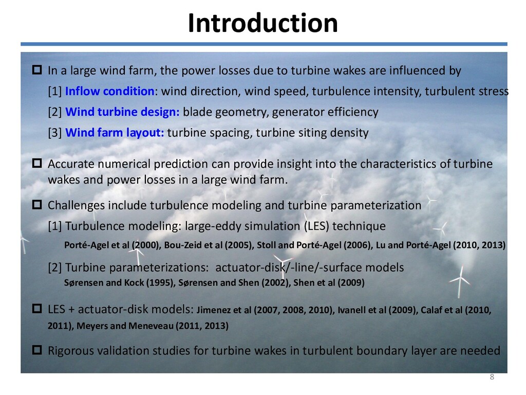
8. Introduction  In a large wind farm, the power losses due to turbine wakes are influenced by [1] Inflow condition: wind direction, wind speed, turbulence intensity, turbulent stress [2] Wind turbine design: blade geometry, generator efficiency [3] Wind farm layout: turbine spacing, turbine siting density  Accurate numerical prediction can provide insight into the characteristics of turbine wakes and power losses in a large wind farm.  Challenges include turbulence modeling and turbine parameterization  LES + actuator-disk models: Jimenez et al (2007, 2008, 2010), Ivanell et al (2009), Calaf et al (2010, 2011), Meyers and Meneveau (2011, 2013) [1] Turbulence modeling: large-eddy simulation (LES) technique [2] Turbine parameterizations: actuator-disk/-line/-surface models Porté-Agel et al (2000), Bou-Zeid et al (2005), Stoll and Porté-Agel (2006), Lu and Porté-Agel (2010, 2013) Sørensen and Kock (1995), Sørensen and Shen (2002), Shen et al (2009) 8  Rigorous validation studies for turbine wakes in turbulent boundary layer are needed
9. Rough terrain (forest) Less rough (prairie) Smooth surface (sea surface) Wu and Porté-Agel (2012)
10. Rough terrain (forest) Less rough (prairie) Smooth surface (sea surface) Wu and Porté-Agel (2012) How far the downstream turbines should be installed
11. Solution Numerical modelling Laboratory experiment Field campaign
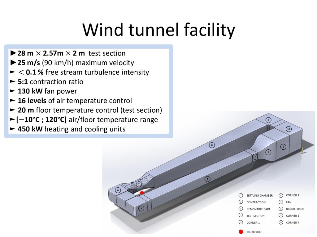
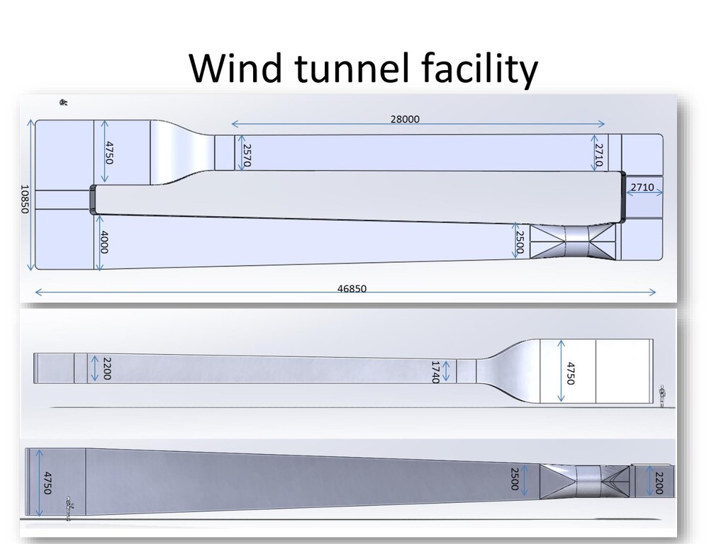
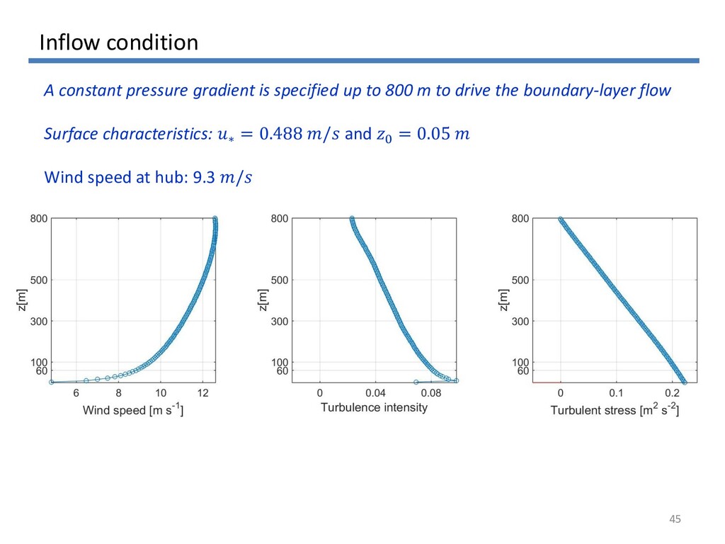
12. Wind tunnel facility ►28 m × 2.57m × 2 m test section ►25 m/s (90 km/h) maximum velocity ► < 0.1 % free stream turbulence intensity ► 5:1 contraction ratio ► 130 kW fan power ► 16 levels of air temperature control ► 20 m floor temperature control (test section) ►[−10°C ; 120°C] air/floor temperature range ► 450 kW heating and cooling units
13. Wind tunnel facility
17. Wind measurements Meteorological Masts Remote-sensing Measurements (e.g., LIDAR, SODAR) 17
18. Meteorological Masts 18
19. 台電離岸式測風塔 19
21. 海氣象觀測塔設備 氣象儀器 儀器 項目 風速計 風向計 大氣壓力計 溫溼度計 雨量計 日輻射儀 廠牌-型號 Thies 4.3351.10.000 Thies 4.3150.10.400 Thies 3.1157.10.000 Driesen+Kern Gmbh DKRF400 Campbell TE525MM Kipp&Zonen CNR4 規格 範圍 0.3~70 m/s 0~360° 300~1100 mb -40~+80°C 0~100% RH 4.73 ml/tip 300 to 2800 nm 4.5 to 42 μm 解析度 0.05 m wind run 0.1° 0.01hPa 0.01°C 0.05% 0.1 mm/tip 0.01 w/m2 精度 < 0.2 m/s 1° ± 0.25 hPa ±0.3°C ±1.8%RH ±1% <1% 安裝於塔架 位置(數量) EL+95m(2) EL+50m(1) EL+30m(1) EL+10m(1) EL+95m(1) EL+50m(1) EL+30m(1) EL+10m(1) EL+95m(1) EL+10m(1) EL+95m(1) EL+10m(1) EL+10m(1) EL+19m(1)
23. LIDAR(光達) • LIDAR: Light Detection And Ranging 23 3D scanning LIDAR Galion HALO Photonics WindCube
24. LIDAR(光達) • HALO Photonics 3D scanning LIDAR 24
25. LIDAR(光達) • LIDAR: Light Detection And Ranging 25 Profiling LIDAR
26. Light Doppler shift − 0 0 = = Observed wavelength = Emitted velocity of light source = Speed of light 0 = Rest emitted wavelength Eq: Observer Source
27. WindSentinel  Floating LiDAR device by AXYS  Buoy System (Vindicator, Anemometers, Solar Panels, Turbines, Batteries, etc)  Vindicator by OADS (Optical Air Data Systems )
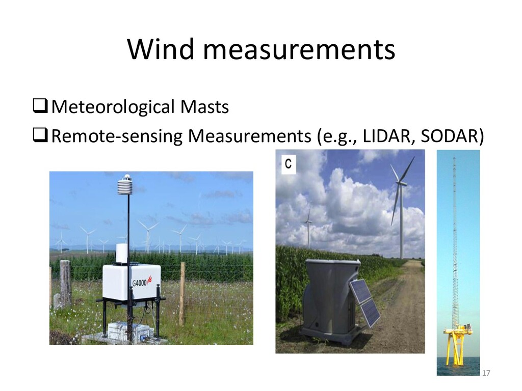
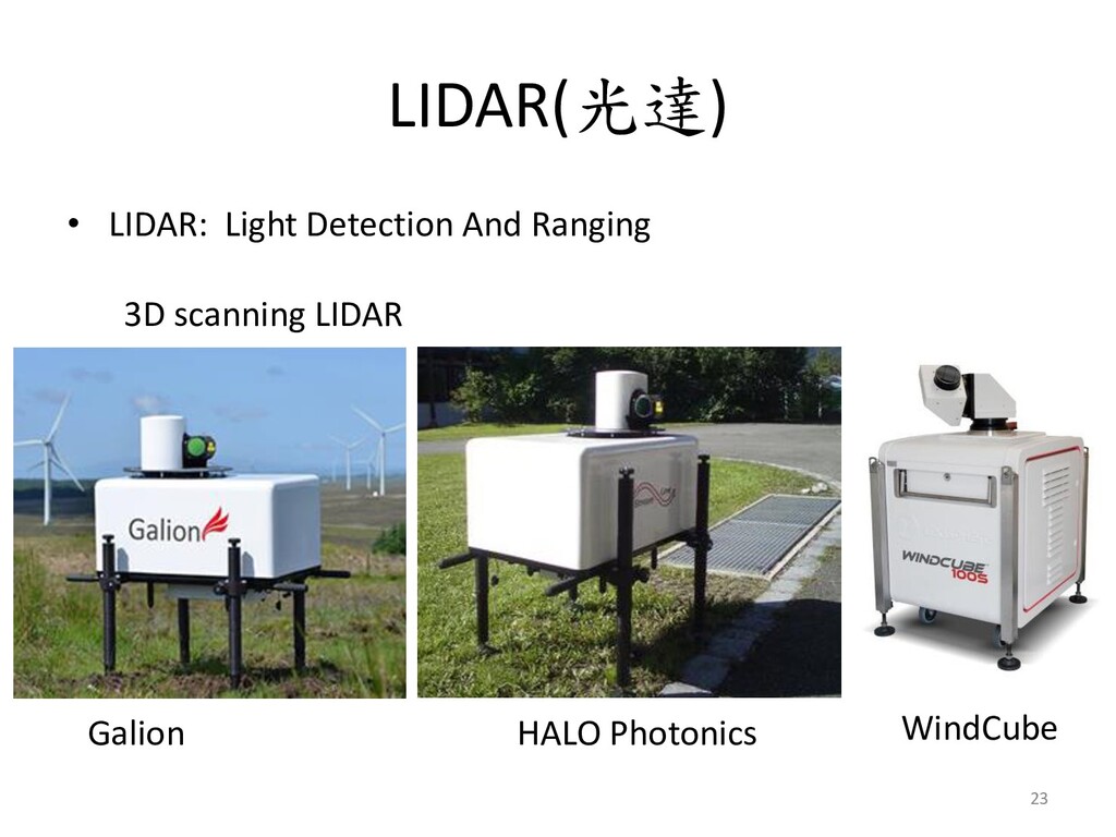
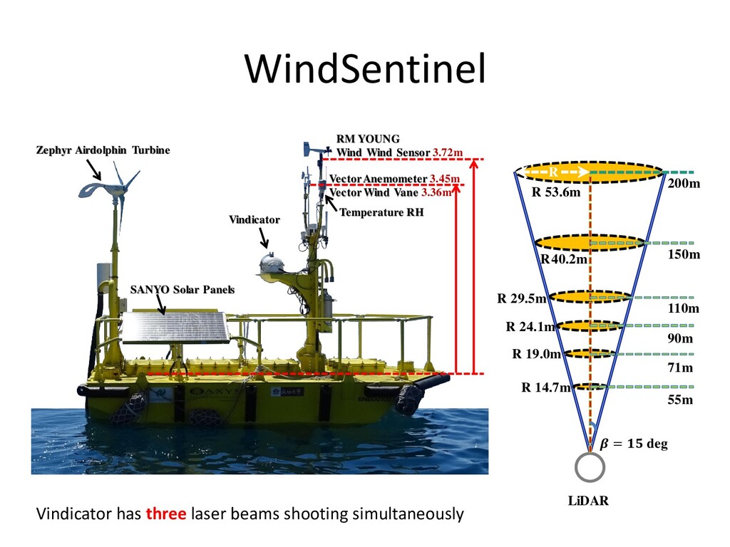
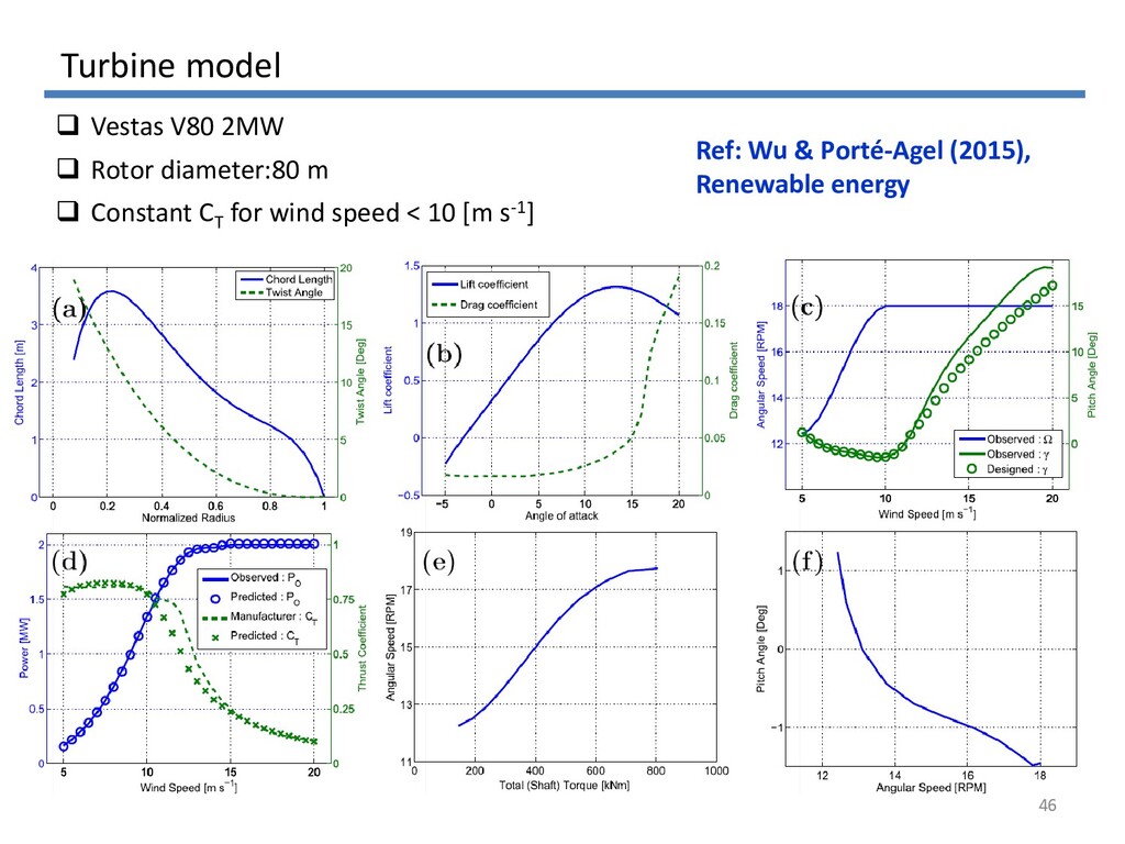
28. WindSentinel RM YOUNG Wind Wind Sensor 3.72m Zephyr Airdolphin Turbine SANYO Solar Panels Vector Anemometer 3.45m Vector Wind Vane 3.36m Temperature RH Vindicator 55m 71m 90m 110m 150m 200m = deg R 53.6m R40.2m R 29.5m R 24.1m R 19.0m R 14.7m R LiDAR Vindicator has three laser beams shooting simultaneously
29. WindSentinel 1 (1 ) 2 (2 ) 3 (3 ) Buoy LIDAR 1 2 3 = sin 1 cos 1 1 sin 2 cos 2 1 sin 3 cos 3 1 sin 0 0 0 sin 0 0 0 cos ⟹ 1 2 3 = ⟹ = = −1 1 2 3
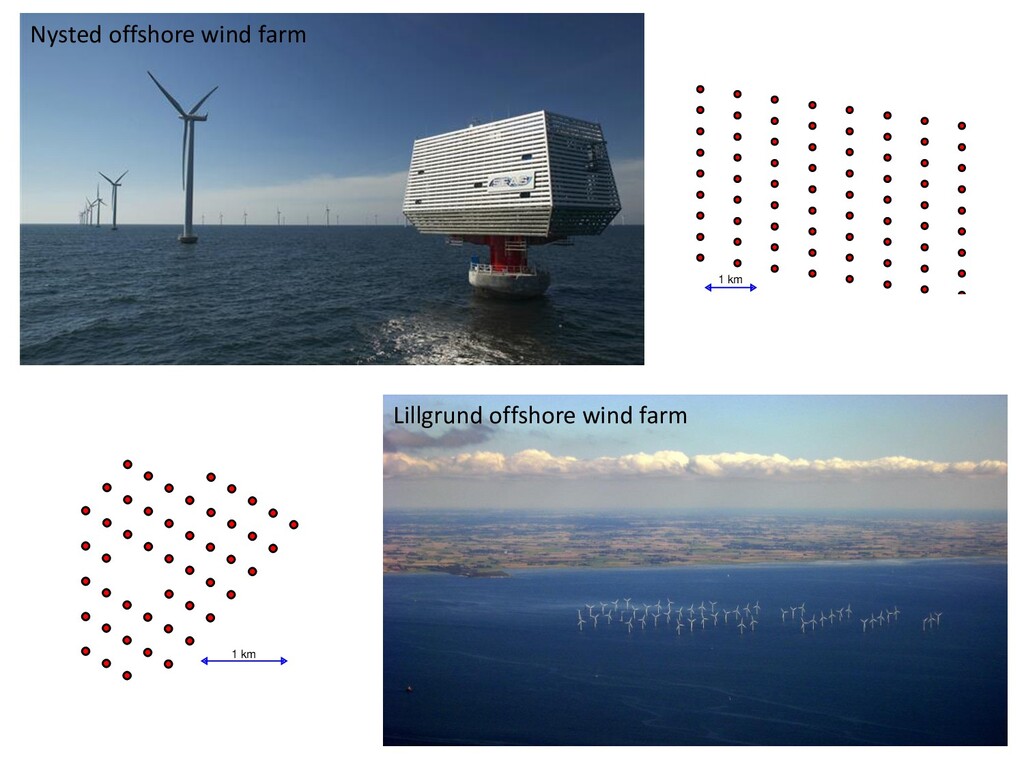
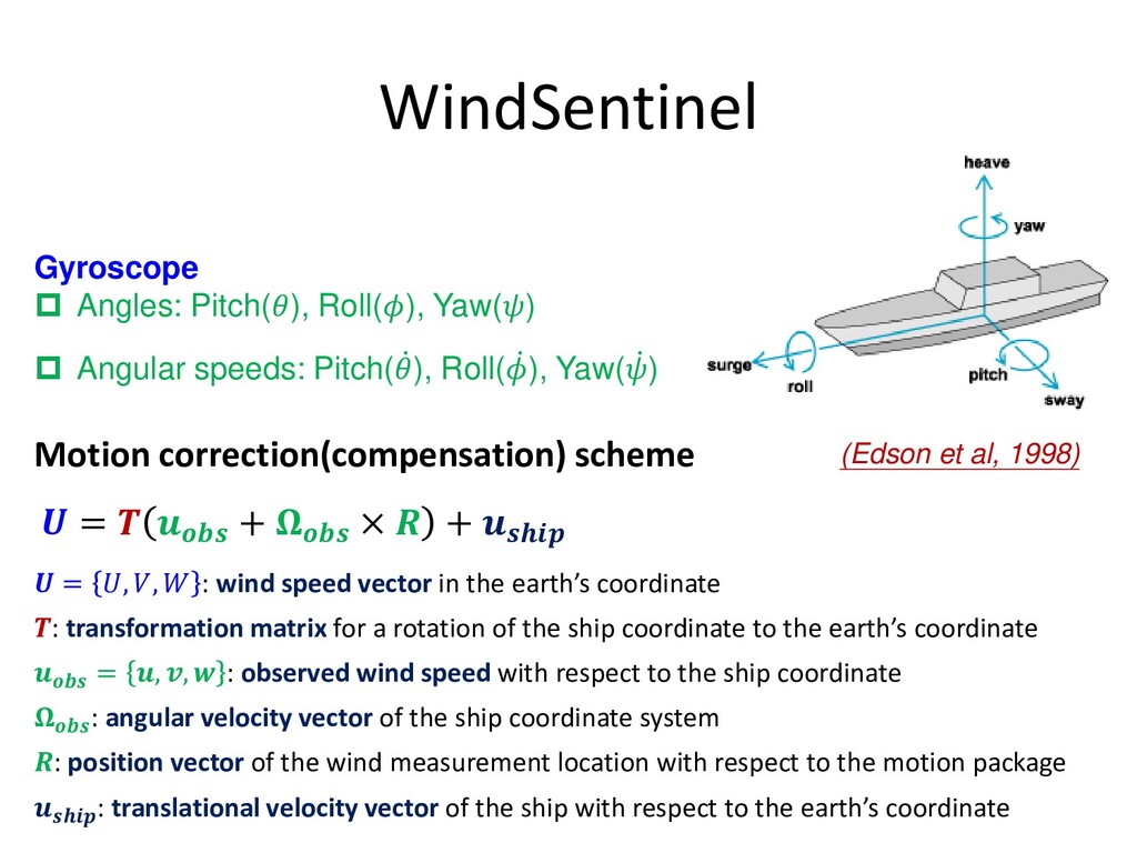
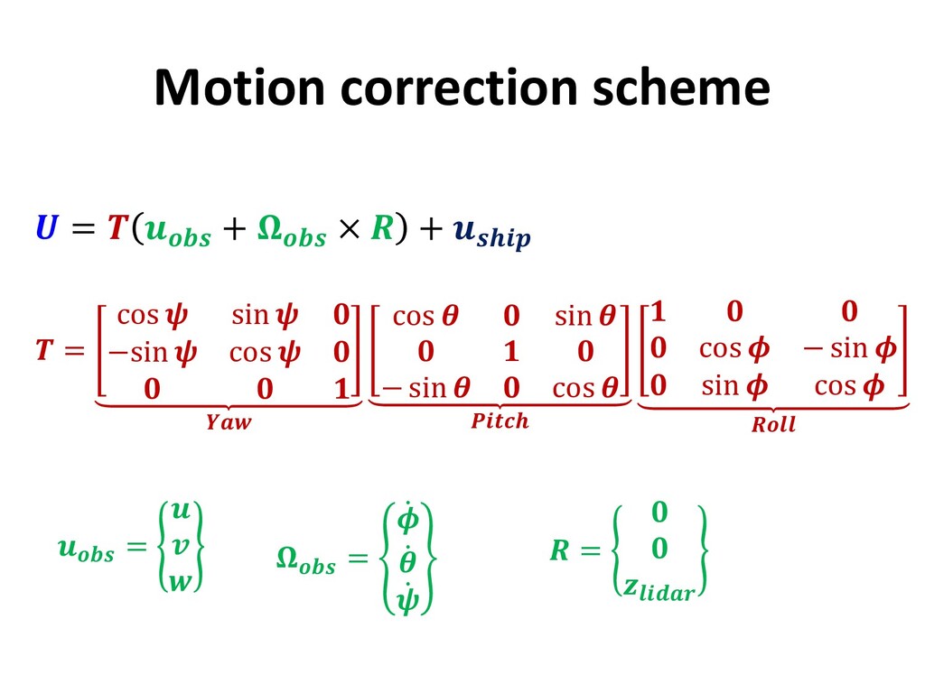
30. WindSentinel Gyroscope  Angles: Pitch(), Roll(), Yaw()  Angular speeds: Pitch( ሶ ), Roll( ሶ ), Yaw( ሶ ) = + × + Motion correction(compensation) scheme (Edson et al, 1998) = , , : wind speed vector in the earth’s coordinate : transformation matrix for a rotation of the ship coordinate to the earth’s coordinate : angular velocity vector of the ship coordinate system : position vector of the wind measurement location with respect to the motion package : translational velocity vector of the ship with respect to the earth’s coordinate = , , : observed wind speed with respect to the ship coordinate
31. Motion correction scheme = + × + = cos sin −sin cos cos sin − sin cos cos − sin sin cos = = ሶ ሶ ሶ =
32. Large-eddy simulation framework ෤ = 0 ෤ + ෤ ෤ − ෤ = − ෤ ∗ − + 2 ෤ 2 − + 1 : air kinematic viscosity : modified pressure : resolved (filtered) velocity : a filter scale (Δ) ~ ෤ ෤ ∗ : subgrid-scale (SGS) stress : turbine-induced body forces : constant pressure gradient i
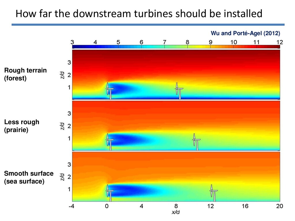
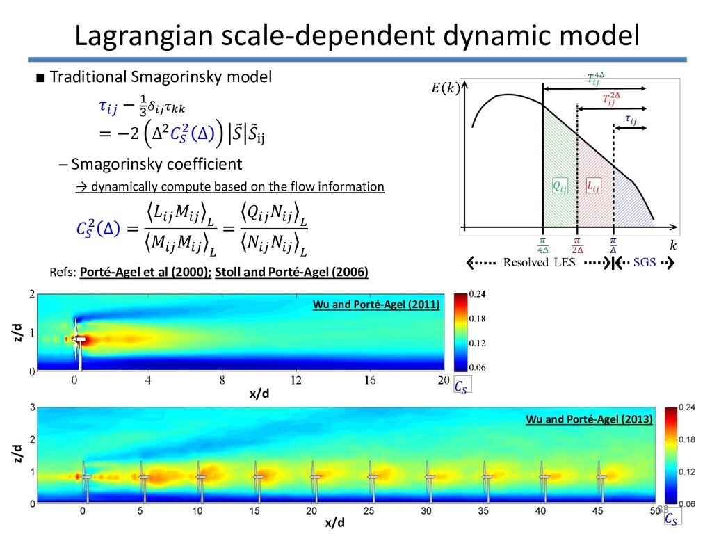
33. Lagrangian scale-dependent dynamic model − 1 3 = −2 Δ2 2 Δ ሚ ሚ ij 2 Δ = = ▪ Traditional Smagorinsky model ̶ Smagorinsky coefficient → dynamically compute based on the flow information Refs: Porté-Agel et al (2000); Stoll and Porté-Agel (2006) z/d z/d x/d x/d Wu and Porté-Agel (2011) Wu and Porté-Agel (2013) 33
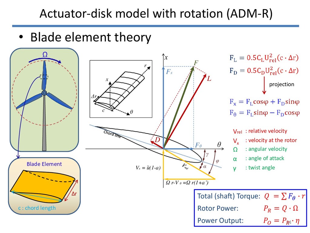
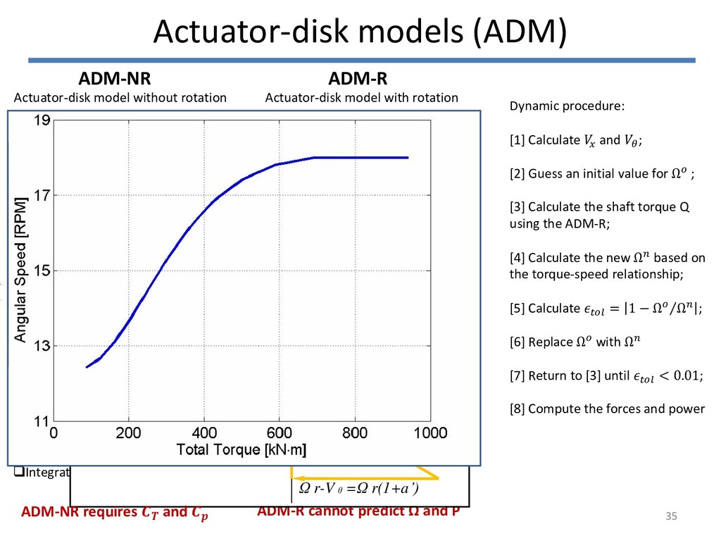
34. Ω • Blade element theory Δr c : chord length Blade Element Vrel : relative velocity Vx : velocity at the rotor Ω : angular velocity α : angle of attack γ : twist angle projection Total (shaft) Torque: = σ ∙ Rotor Power: = ∙ Ω Power Output: = ∙ Ω r-V θ =Ω r(1+a’) L D Fx Fθ θ α φ γ F Vx = u(1-a) ~ x r θ x c Δr Actuator-disk model with rotation (ADM-R) 34
35. ADM-NR ADM-R Uniform distribution of thrust No considering rotation effect Integrating thrust force over time Non-uniform distribution of thrust Considering rotation effect Integrating the forces over time Actuator-disk model without rotation Actuator-disk model with rotation Jimenez et al (2007; 2008) Calaf et al (2010; 2011) Wu & Porté-Agel (2011, 2013) Sørensen & Kock (1995) Kasmi & Masson (2008) Wu & Porté-Agel (2011, 2013) Blade element theory 1D momentum theory Actuator-disk models (ADM) ADM-R cannot predict Ω and P Dynamic procedure: [1] Calculate and ; [2] Guess an initial value for Ω ; [3] Calculate the shaft torque Q using the ADM-R; [4] Calculate the new Ω based on the torque-speed relationship; [5] Calculate = 1 − Τ Ω Ω ; [6] Replace Ω with Ω [7] Return to [3] until < 0.01; [8] Compute the forces and power Ω r-V θ =Ω r(1+a’) L D Fx Fθ θ α φ γ F Vx = u(1-a) ~ x r θ x c Δr ADM-NR requires and 35
36. Model validation Horns Rev offshore wind farm (Wu and Porte-Agel, 2015) A model wind farm in ABL wind tunnel (Wu and Porte-Agel, 2013)
37. U [m s-1] LES+ADM-R 37 Grid number: × × CPU cores: 256 cores Computational time: 24 hours Simulation time: 80 mins LES of turbine wakes in the Horns Rev offshore wind farm
38. Model validation: farm power prediction Horns Rev offshore wind farm  Wind farm area : 20 [km2]  80 Vestas V80 2MW wind turbines  Total wind farm output: 160 MW  Cut-in wind speed: 4 [m s-1]  Cut-out wind speed: 25 [m s-1]  Constant CT for wind speed < 10 [m s-1]  Rotor diameter (d) = 80 [m]  Turbine hub height (HHUB ) = 70 [m]  Three masts around the farm 5 8 11 14 17 20 0 0.5 1 1.5 2 Power [MW] Wind Speed [ms-1] 5 8 11 14 17 20 0 0.25 0.5 0.75 1 Thrust Coefficient Measured Power Manufacturers C T (Hansen et al, 2012) From: Fredy Rodriguez @ http://vimeo.com/28745771 38
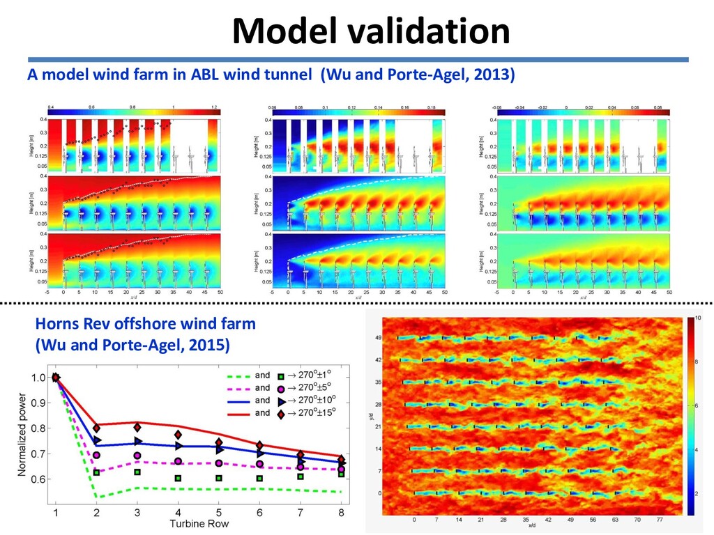
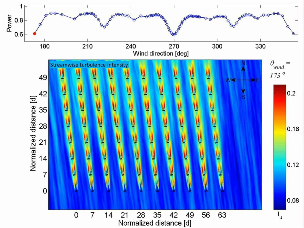
39. U [m s-1] Yaw misalignment is ignored in the sorting of the observed power data, which can cause an overestimation on the power output of downstream turbines in a narrow full wake condition (e.g. 270o±1o). Lines: simulated power Symbols: measured power Power prediction for different wind sectors
40. Time-averaged streamwise velocity
41. Streamwise turbulence intensity
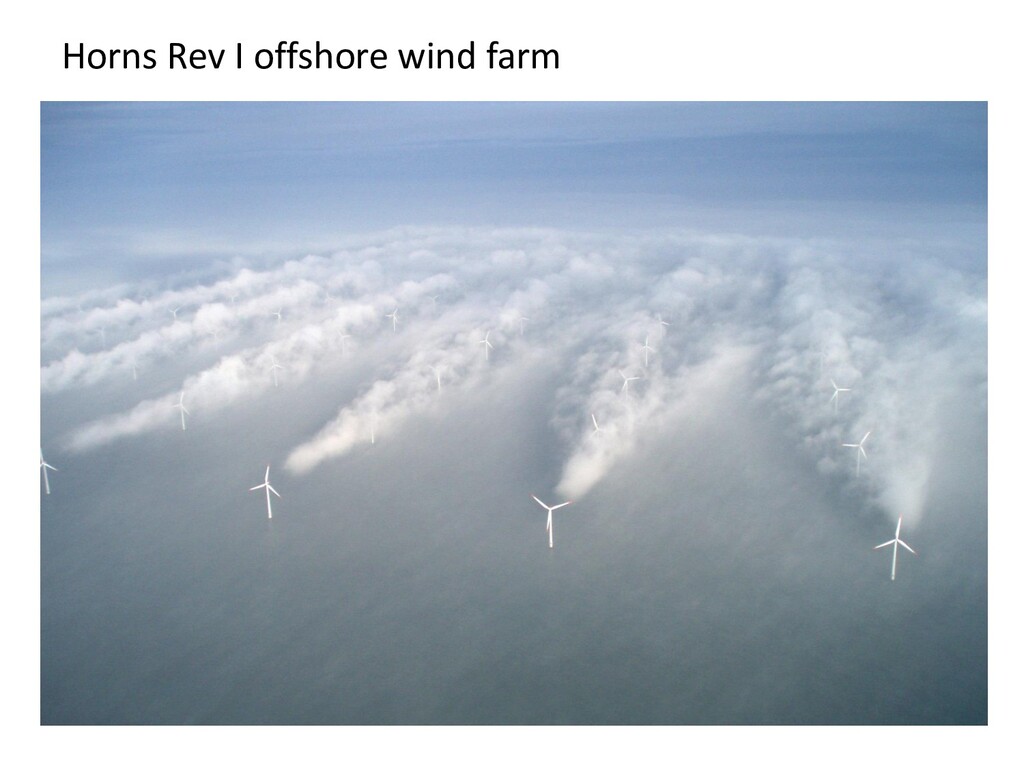
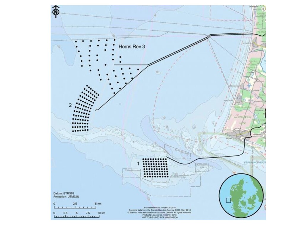
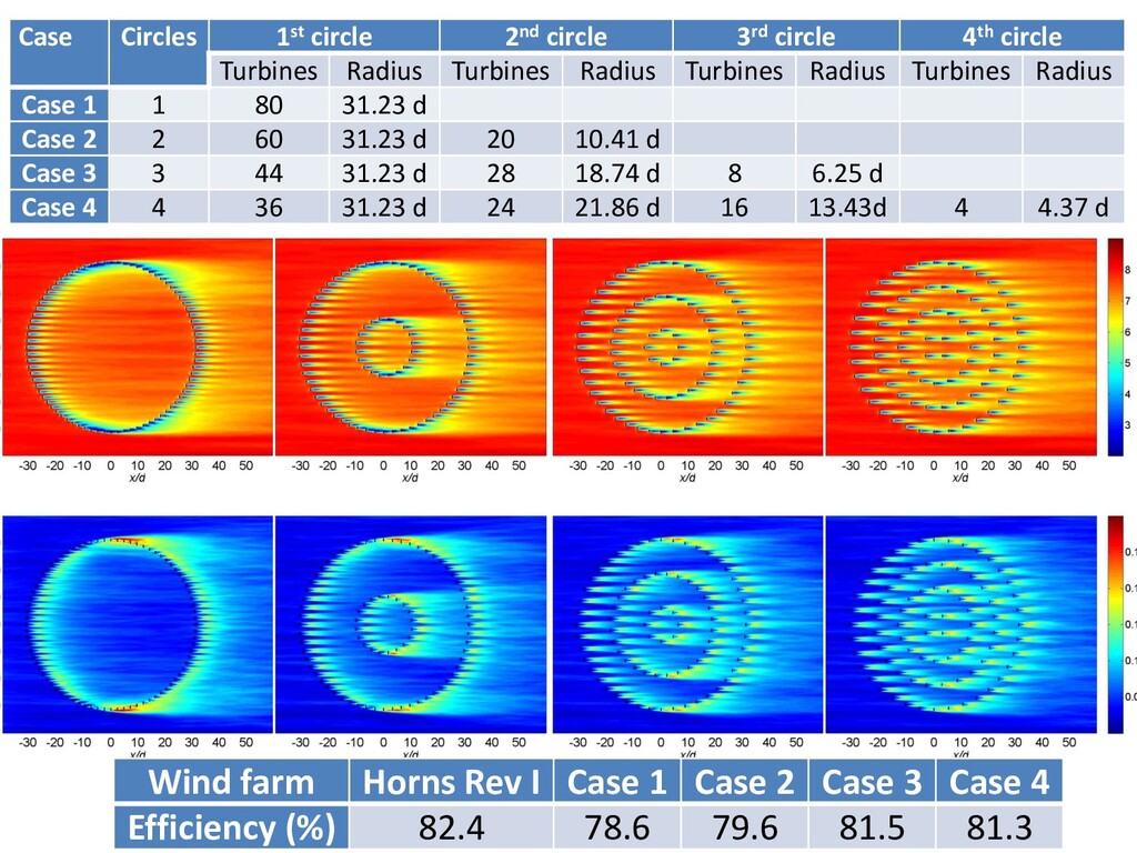
43. Case Circles 1st circle 2nd circle 3rd circle 4th circle Turbines Radius Turbines Radius Turbines Radius Turbines Radius Case 1 1 80 31.23 d Case 2 2 60 31.23 d 20 10.41 d Case 3 3 44 31.23 d 28 18.74 d 8 6.25 d Case 4 4 36 31.23 d 24 21.86 d 16 13.43d 4 4.37 d Wind farm Horns Rev I Case 1 Case 2 Case 3 Case 4 Efficiency (%) 82.4 78.6 79.6 81.5 81.3
44. Simulations of large wind farms 44 = 24,000 = 300 = 1,200 = 15 = 996.8 = 12.5 120 wind turbines are sited in the simulations = 1,200 = 192 = 160
45. Inflow condition 45 A constant pressure gradient is specified up to 800 m to drive the boundary-layer flow Surface characteristics: ∗ = 0.488 / and 0 = 0.05 Wind speed at hub: 9.3 /
46. Turbine model 46  Vestas V80 2MW  Rotor diameter:80 m  Constant CT for wind speed < 10 [m s-1] Ref: Wu & Porté-Agel (2015), Renewable energy
47. Simulated power output 47 0.50 0.55 0.60 0.65 0.70 0.75 0.80 WF1 WF2 WF3 WF4 WF5 WF6 WF7 WF8 Average Power (1-10) Average Power (11-20) Average Power (21-30) Average Power (1-30)
49. Averaged streamwise velocity 49
51. Published: Wu et al, Renewable Energy, 2019
52. Lu & Porté-Agel (2011) Thanks for your attention Q&A