3D colored mesh structure-preserving filtering with adaptive p-Laplacian on directed graphs

Transcript

1. 3D colored mesh structure-preserving filtering with adaptive p-Laplacian on directed graphs S´ ebastien Bougleux1, Olivier L´ ezoray1, Anass Nouri2 1Normandie Univ, UNICAEN, ENSICAEN, CNRS, GREYC, 14000 Caen, France 2Vision Lab. Isen Brest, L@bISEN, 29228 Brest Cedex, France olivier.lezoray@unicaen.fr https://lezoray.users.greyc.fr
2. 1 Introduction 2 p-Laplacian on directed graphs 3 Adaptive p-Laplacian structure preserving filtering 4 Results 5 Conclusion 2 / 23
3. 1 Introduction 2 p-Laplacian on directed graphs 3 Adaptive p-Laplacian structure preserving filtering 4 Results 5 Conclusion 3 / 23
4. Introduction Recent technological advances have led to the generation of huge amounts of 3D data Even with cheap hardware and software, on can easily generate 3D colored meshes Strong demand of algorithms for the editing of 3D colored meshes (for simplification, sharpness enhancement, etc.) 4 / 23
5. Example of low-quality 3D color scan editing Statue scanned with a NextEngine 3DScanner (cheap) 5 / 23
6. Example of low-quality 3D color scan editing → Statue scanned with a NextEngine 3DScanner (cheap) (left: original, right: enhanced). 5 / 23
7. Structure-preserving filtering For images : state-of-the-art editing approaches consider structure-preserving smoothing filters within a hierarchical framework An image is decomposed into several layers from coarse to fine details Very few approaches have addressed this problem for the editing 3D colored meshes Our proposal : a structure-preserving filter with adaptive p-Laplacian on directed graphs 6 / 23
8. 1 Introduction 2 p-Laplacian on directed graphs 3 Adaptive p-Laplacian structure preserving filtering 4 Results 5 Conclusion 7 / 23
9. Graph signals We consider 3D colored signals defined on a domain represented by a graph (a triangulated mesh). A graph G = (V, E) consists in a set V = {v1, . . . , vnv } of vertices and a set E ⊂ V × V of edges connecting vertices. A graph signal is a function that associates real-valued vectors to vertices of the graph f : G → Rnc . The graph signal of nv elements is represented by a real matrix F = [fi,c ]i∈Nv ,c∈Nc , with Nv = {1, . . . , nv } and Nc = {1, . . . , nc } The i-th element can be represented by a vector fi = [fi,c ]c∈Nc The graph is represented by its weighted vertex-vertex adjacency matrix W = [wi,j ]i∈Nv ,j∈Nv , with wi,j ∈ (0, +∞) We consider directed graphs and wi,j ∈ E does not imply that wj,i ∈ E 8 / 23
10. p-Laplacian on directed graphs We have recently proposed several formulations for the p-Laplacian on directed graphsa. We consider here the unnormalized case aZ. Abu-Aisheh, S. Bougleux, O. L´ ezoray, p-Laplacian regularization of signals on directed graphs, International Symposium on Visual Computing, Vol. LNCS 11241, pp. 650-661, 2018 The Gradient Gradient of a graph signal F is given by ∇WF = (∂W j F)j∈Nv , with ∂W j F = [ √ wi,j (fj,c − fi,c )]i∈Nv ,c∈Nc the directional differences according to vertex j The gradient at a vertex i is thus given by ∇W i F = [ √ wi,j (fj,c − fi,c )]j∈Nv ,c∈Nc Its norm is given by |∇W i F| = nv j=1 wi,j nc c=1 (fj,c − fi,c )2 9 / 23
11. p-Laplacian on directed graphs The regularity of the graph signal F is given by its p-total variation F pTV = |∇WF|p 1 = nv i=1 |∇W i F|p where p ∈ [1, +∞) controls the degree of regularity. The p-Laplacian The (directed) p-Laplacian is given by Lp,F = diag((Wp,F + WT p,F )1nv ) − (Wp,F + WT p,F ) with Wp,F = diag(|∇WF|p−2)W Can be rewritten as [Lp,F F]i,c = nv j=1 wi,j |∇W i F|2−p + wj,i |∇W j F|2−p (fi,c − fj,c ) One can show that ∇ F pTV = p Lp,F F For p = 2, L2,F = L and for p = 1, L1,F F defines the weighted (mean) curvature of F The p-Laplacian is non-linear, and can be viewed as a data-dependent Laplacian 10 / 23
12. 1 Introduction 2 p-Laplacian on directed graphs 3 Adaptive p-Laplacian structure preserving filtering 4 Results 5 Conclusion 11 / 23
13. Objective formulation We propose a structure-preserving smoothing filter based on an adaptive p-Laplacian and a guided preservation of gradient magnitudes. arg min F∈Rn×3 λd F − F0 2 fidelity + λs Es (F, F0, α, S) structures + λr Er (F, F0, p, W) regularity with an initial graph signal F0 = (fi,c )i,c ∈ Rn×3 (colors) and two graphs S and W (same structure but different weights). Structure Preservation: Es (F, F0, α, S) := 1 2N n i=1 αi |∇S i F|2 − |∇S i F0|2 2 guided by α = (αi )n i=1 ∈ [0, 1]n indicating ± the presence of structures on the non weighted directed graph S constructed from the mesh S0 Adaptive pTV regularization: Er (F, F0, p, W) := n i=1 1 pi ∇W i F pi p = (pi )n i=1 ∈ [1, 2]n is the regularity degree of each vertex p depends on F0, opposite role to α, indicating ± the abscence of structures on the weighted directed graph W constructed from S0 12 / 23
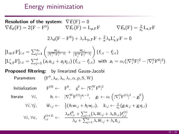
14. Energy minimization Resolution of the system: ∇E(F) = 0 ∇Ed (F) = 2(F − F0) ∇Er (F) = Lp,F F ∇Es (F) = 2 ns Ls,F F 2λd (F − F0) + λr Lp,F F + 2 n λsLs,F F = 0 [Lp,F F]i,c = nv j=1 wi,j |∇W i F|2−pi + wj,i |∇W j F|2−pj (fi,c − fj,c ) [Ls,F F]i,c = n j=1 (ai si,j + aj sj,i ) (fi,c − fj,c ) with ai = αi (|∇S i F|2 − |∇S i F0|2) Proposed filtering: by linearized Gauss-Jacobi Parameters (F0, λd , λs , λr , α, p, S, W) Initialization F(0) ← F0, g0 ← |∇W i F0|2 Iterate ∀i, hi ← |∇W i F(t)|pi −2, gi ← αi |∇S i F(t)|2 − g0 i ∀i, ∀j, wi,j ← 1 2 (hi wi,j + hj wj,i ), si,j ← 1 ns (gi si,j + gj sj,i ) ∀i, ∀c, f (t+1) i,c ← λd f 0 i,c + n j=1 (λr wi,j + λs si,j )f (t) j,c λd + n j=1 λr wi,j + λs si,j 13 / 23
15. Construction of the graphs Performed by comparing the features associated to the vertices {vi }nv i=1 « Set of colors Φτ i := (L∗a∗b∗(f0 j ))j∈N τ i (S0)∪{i} with Nτ i (S0) the set of vertices reached from i within a τ-hop in S0 « The Earth Mover Distance between the histograms of Φτ i is used to compare vertices si,j := 1 si j k-nn of i according to dEMD (H(Φτ i ), H(Φτ l )), l ∈ Nβ i (S0) 0 otherwise wi,j := 1 − dEMD (H(Φτ i ), H(Φτ j )) max l=1,...,n si,l =1 dEMD (H(Φτ i ), H(Φτ l )) if si,j = 1, wi,j := 0 otherwise « W and S have the same structure but different weights. « Parameters: τ, β, k ∈ N>0 « The graphs are directed (k-nn) 14 / 23
16. Structure Indicator p and α are defined from a structure indicator m := (mi )n i=1 mi := 1 |N ρ i (S0)| j∈N ρ i (S0) dEMD (H(Φρ−1 i ), H(Φρ−1 j )) pi :=1 + 1 1 + m2 i , αi := mi − minj mj δi (maxj mj − minj mj ) , δi out-degree of i in S « pi and αi are antagonists : one for smoothing the data, the other for preserving the main structures « Parameter: ρ ∈ N>0 15 / 23
17. 1 Introduction 2 p-Laplacian on directed graphs 3 Adaptive p-Laplacian structure preserving filtering 4 Results 5 Conclusion 16 / 23
18. Simple example Initial mesh Structure indicator pi = 2, λs = 0 pi = 1, λs = 0 pi , λs = 0 pi , λs = 0.25 17 / 23
19. Editing example Original 18 / 23
20. Editing example Original Structure Indicator 18 / 23
21. Editing example Original p = 2, λs = 0 18 / 23
22. Editing example Original p = 1, λs = 0 18 / 23
23. Editing example Original pi , λs = 0 18 / 23
24. Editing example Original pi , λs = 0.25 18 / 23
25. Editing example Original pi , λs = 0.25 Sharpening 18 / 23
26. Editing example Original pi , λs = 0.25 Abstraction 18 / 23
27. Editing example Original 19 / 23
28. Editing example Original pi , λs = 0.25 19 / 23
29. Editing example Original Sharpening 19 / 23
30. Editing example Original Abstraction 19 / 23
31. Editing example Original 20 / 23
32. Editing example Original pi , λs = 0.25 20 / 23
33. Editing example Original Sharpening 20 / 23
34. 1 Introduction 2 p-Laplacian on directed graphs 3 Adaptive p-Laplacian structure preserving filtering 4 Results 5 Conclusion 21 / 23
35. Conclusion We have proposed : A structure-preserving filter for graph signals relying on a data-fitting term, a smoothness term and a structure-preserving term The energy is formalized on directed graphs with the p-Laplacian The filtering process is adaptive with is use of a spatially-variant p-Total Variation norm The filtering is guided with a structure indicator to preserve the main structures This enables to Obtain a coarse filtering of 3D colored meshes : rough structures while preserving the edges Perform editing tasks such as sharpening and abstraction 22 / 23
36. The end Publications available at : https://lezoray.users.greyc.fr Fundings from ANR-14-CE27-0001 GRAPHSIP, UE FEDER/FSE 2014/2020 and NVIDIA 23 / 23