ICPR 2020

Transcript

1. GRAPH SIGNAL ACTIVE CONTOURS Olivier L´ EZORAY Normandie Univ, UNICAEN, ENSICAEN, CNRS, GREYC, Caen, FRANCE olivier.lezoray@unicaen.fr https://lezoray.users.greyc.fr
2. Outline . Introduction . Graph Signal Active contours . Results . Conclusion O. L´ ezoray Graph signal active contours /
3. Outline . Introduction . Graph Signal Active contours . Results . Conclusion O. L´ ezoray Graph signal active contours /
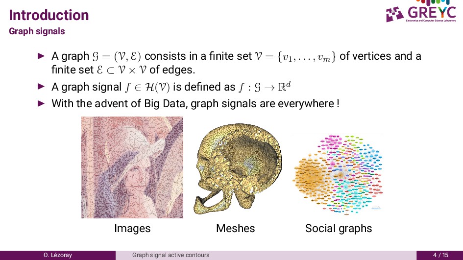
4. Introduction Graph signals A graph G = (V, E) consists in a finite set V = {v1, . . . , vm} of vertices and a finite set E ⊂ V × V of edges. A graph signal f ∈ H(V) is defined as f : G → Rd With the advent of Big Data, graph signals are everywhere ! Images Meshes Social graphs O. L´ ezoray Graph signal active contours /
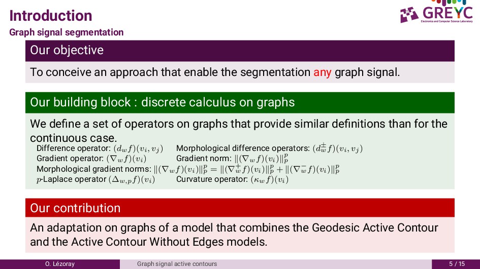
5. Introduction Graph signal segmentation Our objective To conceive an approach that enable the segmentation any graph signal. Our building block : discrete calculus on graphs We define a set of operators on graphs that provide similar definitions than for the continuous case. Difference operator: (dwf)(vi, vj) Morphological difference operators: (d± w f)(vi, vj) Gradient operator: (∇wf)(vi) Gradient norm: (∇wf)(vi) p p Morphological gradient norms: (∇wf)(vi) p p = (∇+ wf)(vi) p p + (∇− w f)(vi) p p p-Laplace operator (∆w,pf)(vi) Curvature operator: (κwf)(vi) Our contribution An adaptation on graphs of a model that combines the Geodesic Active Contour and the Active Contour Without Edges models. O. L´ ezoray Graph signal active contours /
6. Outline . Introduction . Graph Signal Active contours . Results . Conclusion O. L´ ezoray Graph signal active contours 6 /
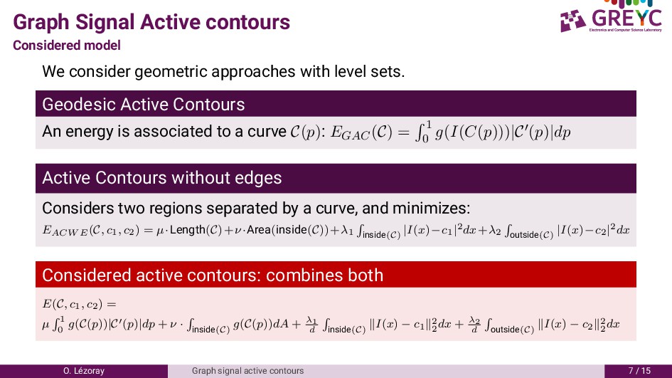
7. Graph Signal Active contours Considered model We consider geometric approaches with level sets. Geodesic Active Contours An energy is associated to a curve C(p): EGAC(C) = 1 0 g(I(C(p)))|C (p)|dp Active Contours without edges Considers two regions separated by a curve, and minimizes: EACW E(C, c1, c2) = µ·Length(C)+ν·Area(inside(C))+λ1 inside(C) |I(x)−c1|2dx+λ2 outside(C) |I(x)−c2|2dx Considered active contours: combines both E(C, c1, c2) = µ 1 0 g(C(p))|C (p)|dp + ν · inside(C) g(C(p))dA + λ1 d inside(C) I(x) − c1 2 2 dx + λ2 d outside(C) I(x) − c2 2 2 dx O. L´ ezoray Graph signal active contours /
8. Graph Signal Active contours Proposed adaptation on graphs Our adaptation We consider local patches Pβ(f, vj) on a β-hop subgraph Bβ(vi) We propose a specific potential function g(vi) that differentiates the most salient structures of a graph using patches comparison We consider average patch-based model to represent the regions (instead of vertex-based signal average) We express front propagation on graphs as δf(vi,t) δt = F(vi) (∇wf)(vi, t) p p with F(vi, t) a speed function. We propose a front propagation function that solves the considered active contours with discrete calculus: F(vi, t) = νg(vi) + µg(vi)(κwf)(vi, t) − λ1 d vi d2(Pβ(fI, vi), Pc1 β (fI)) + λ2 d vi d2(Pβ(fI, vi), Pc2 β (fI)) O. L´ ezoray Graph signal active contours 8 /
9. Outline . Introduction . Graph Signal Active contours . Results . Conclusion O. L´ ezoray Graph signal active contours /
10. Results Grid Graph Signals (a) (b) (c) (d) (e) (f) Figure: From left to right: (a) Original image, (b) Checkerboard initialization, (c) GSAC; g(vi ) = 1, β = 0, (d) g(vi ), (e) GSAC; g(vi ), β = 0, (f) GSAC; g(vi ), β = 1. O. L´ ezoray Graph signal active contours /
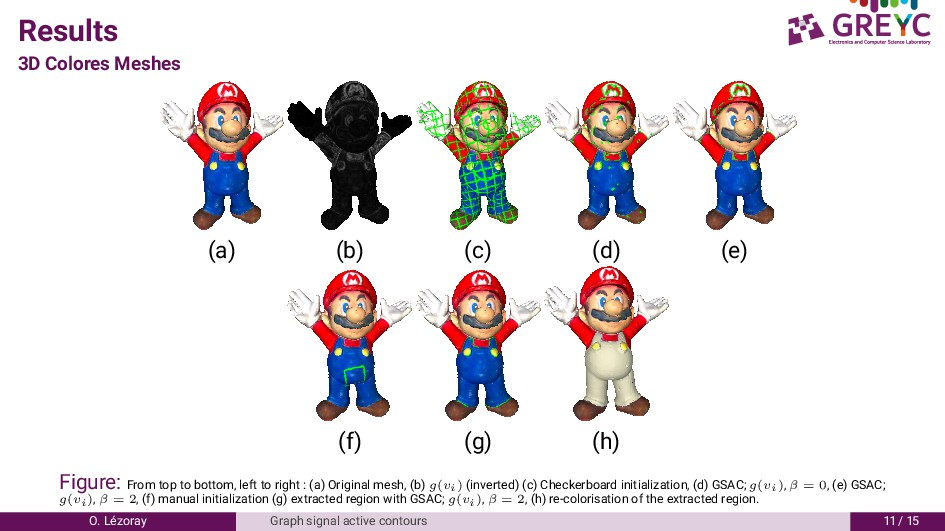
11. Results D Colores Meshes (a) (b) (c) (d) (e) (f) (g) (h) Figure: From top to bottom, left to right : (a) Original mesh, (b) g(vi) (inverted) (c) Checkerboard initialization, (d) GSAC; g(vi), β = 0, (e) GSAC; g(vi), β = 2, (f) manual initialization (g) extracted region with GSAC; g(vi), β = 2, (h) re-colorisation of the extracted region. O. L´ ezoray Graph signal active contours /
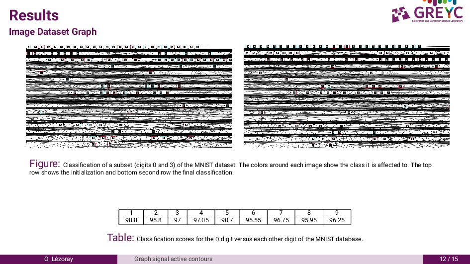
12. Results Image Dataset Graph Figure: Classification of a subset (digits and ) of the MNIST dataset. The colors around each image show the class it is affected to. The top row shows the initialization and bottom second row the final classification. 6 8 8.8 .8 . . . 6. . 6. Table: Classification scores for the 0 digit versus each other digit of the MNIST database. O. L´ ezoray Graph signal active contours /
13. Outline . Introduction . Graph Signal Active contours . Results . Conclusion O. L´ ezoray Graph signal active contours /
14. Conclusion Our contribution Proposed an adaptation of active contours on graphs that combines the Geodesic Active Contour and Active Contours Without Edges approaches A level-set formulation has been adapted on graphs with a framework of graph operators that can describe the evolution of a front on a graph We incorporate specific graph features extracted in the form of a potential function and local graph patches to enhance the segmentation Presented many results on various graph signals Future works Multi-label extension using Voronoi Implicite Interface Model O. L´ ezoray Graph signal active contours /
15. The End Publications available at : https://lezoray.users.greyc.fr Fundings from Saint-Lo Agglo and NVIDIA O. L´ ezoray Graph signal active contours /