IWSSIP 2017

Transcript

1. Stochastic spectral-spatial permutation ordering combination for nonlocal morphological processing Olivier L´ ezoray Normandie Univ, UNICAEN, ENSICAEN, CNRS, GREYC, 14000 Caen, France olivier.lezoray@unicaen.fr https://lezoray.users.greyc.fr
2. 1 Introduction 2 One dimensional permutation ordering 3 Spectral-spatial permutation and consensus ordering 4 Results 5 Conclusion 2 / 27
3. 1 Introduction 2 One dimensional permutation ordering 3 Spectral-spatial permutation and consensus ordering 4 Results 5 Conclusion 3 / 27
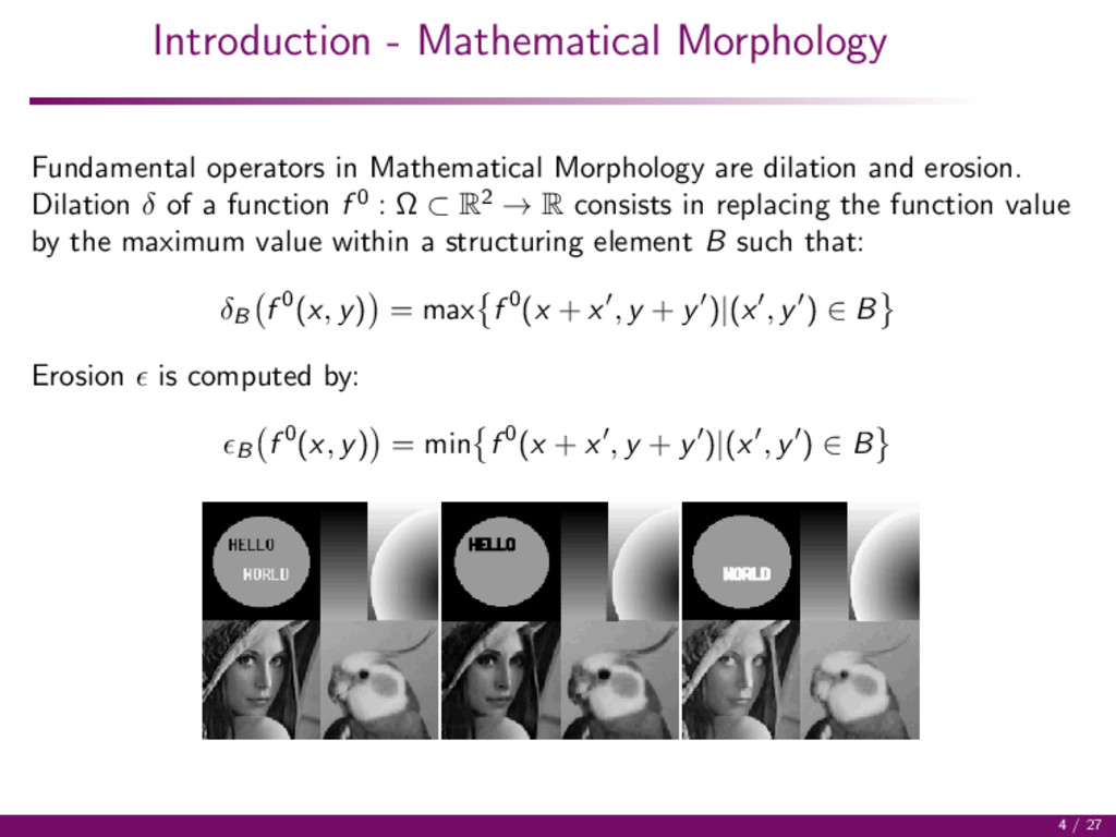
4. Introduction - Mathematical Morphology Fundamental operators in Mathematical Morphology are dilation and erosion. Dilation δ of a function f 0 : Ω ⊂ R2 → R consists in replacing the function value by the maximum value within a structuring element B such that: δB f 0(x, y) = max f 0(x + x , y + y )|(x , y ) ∈ B Erosion is computed by: B f 0(x, y) = min f 0(x + x , y + y )|(x , y ) ∈ B 4 / 27
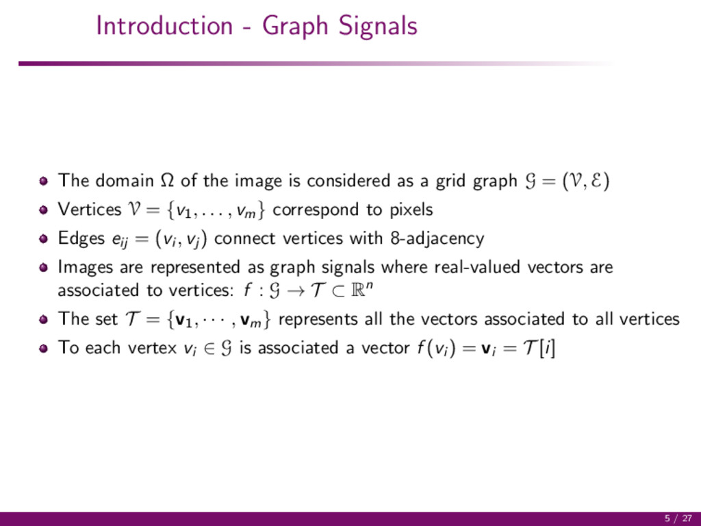
5. Introduction - Graph Signals The domain Ω of the image is considered as a grid graph G = (V, E) Vertices V = {v1, . . . , vm} correspond to pixels Edges eij = (vi , vj ) connect vertices with 8-adjacency Images are represented as graph signals where real-valued vectors are associated to vertices: f : G → T ⊂ Rn The set T = {v1, · · · , vm} represents all the vectors associated to all vertices To each vertex vi ∈ G is associated a vector f (vi ) = vi = T [i] 5 / 27
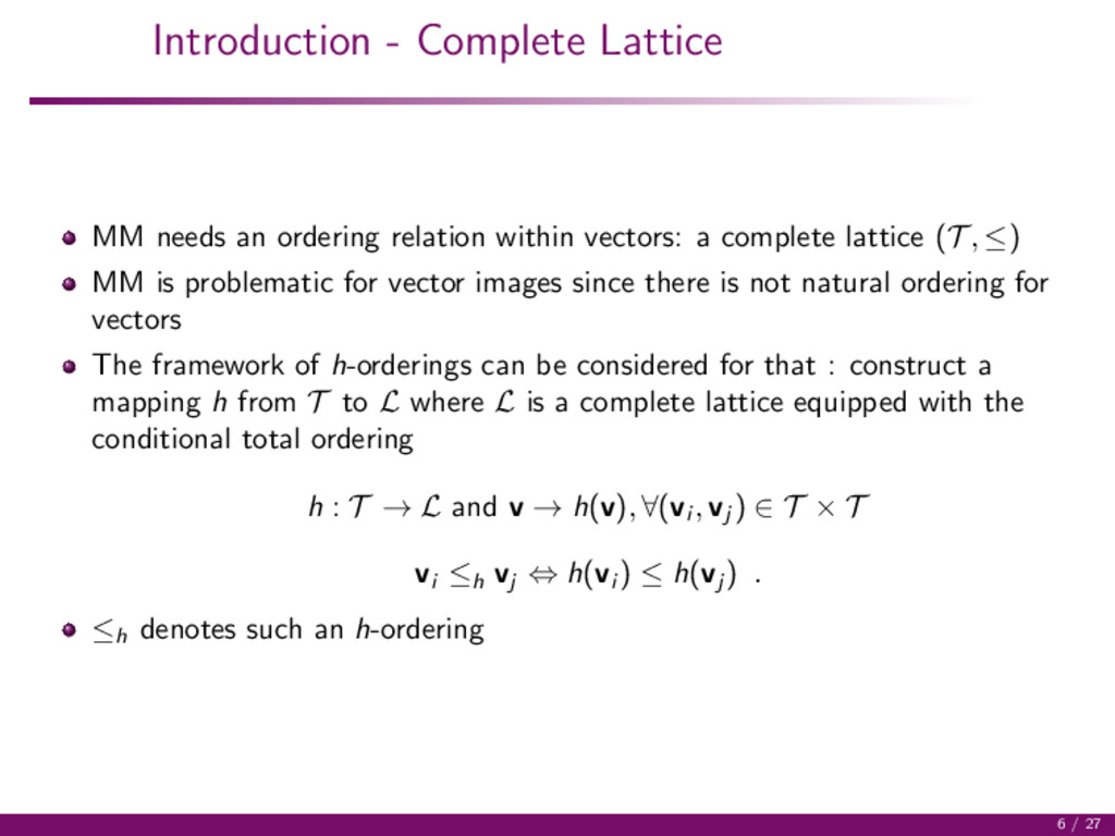
6. Introduction - Complete Lattice MM needs an ordering relation within vectors: a complete lattice (T , ≤) MM is problematic for vector images since there is not natural ordering for vectors The framework of h-orderings can be considered for that : construct a mapping h from T to L where L is a complete lattice equipped with the conditional total ordering h : T → L and v → h(v), ∀(vi , vj ) ∈ T × T vi ≤h vj ⇔ h(vi ) ≤ h(vj ) . ≤h denotes such an h-ordering 6 / 27
7. Introduction - This work Proposes an image-adaptive ordering Takes into account spatial and spectral information to construct the complete lattice (T , ≤h ) Considers several complete lattices and combines them Can benefit from several graph constructions and vector distances Naturally extends to nonlocal processing 7 / 27
8. 1 Introduction 2 One dimensional permutation ordering 3 Spectral-spatial permutation and consensus ordering 4 Results 5 Conclusion 8 / 27
9. 1 Introduction 2 One dimensional permutation ordering 3 Spectral-spatial permutation and consensus ordering 4 Results 5 Conclusion 9 / 27
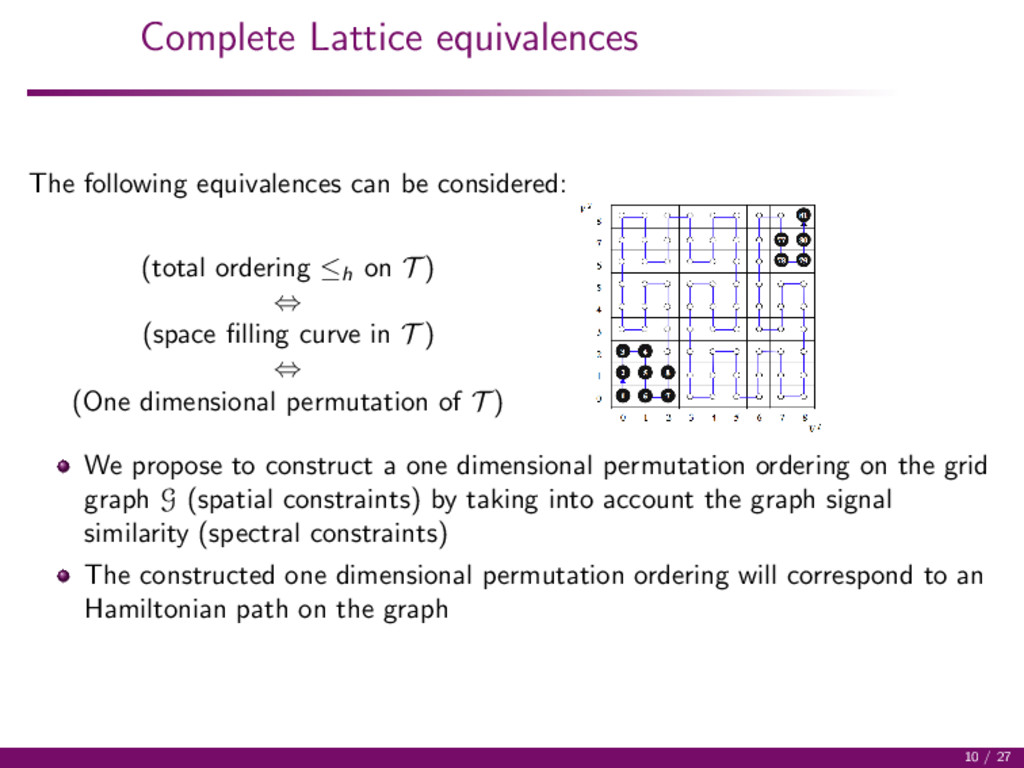
10. Complete Lattice equivalences The following equivalences can be considered: (total ordering ≤h on T ) ⇔ (space filling curve in T ) ⇔ (One dimensional permutation of T ) We propose to construct a one dimensional permutation ordering on the grid graph G (spatial constraints) by taking into account the graph signal similarity (spectral constraints) The constructed one dimensional permutation ordering will correspond to an Hamiltonian path on the graph 10 / 27
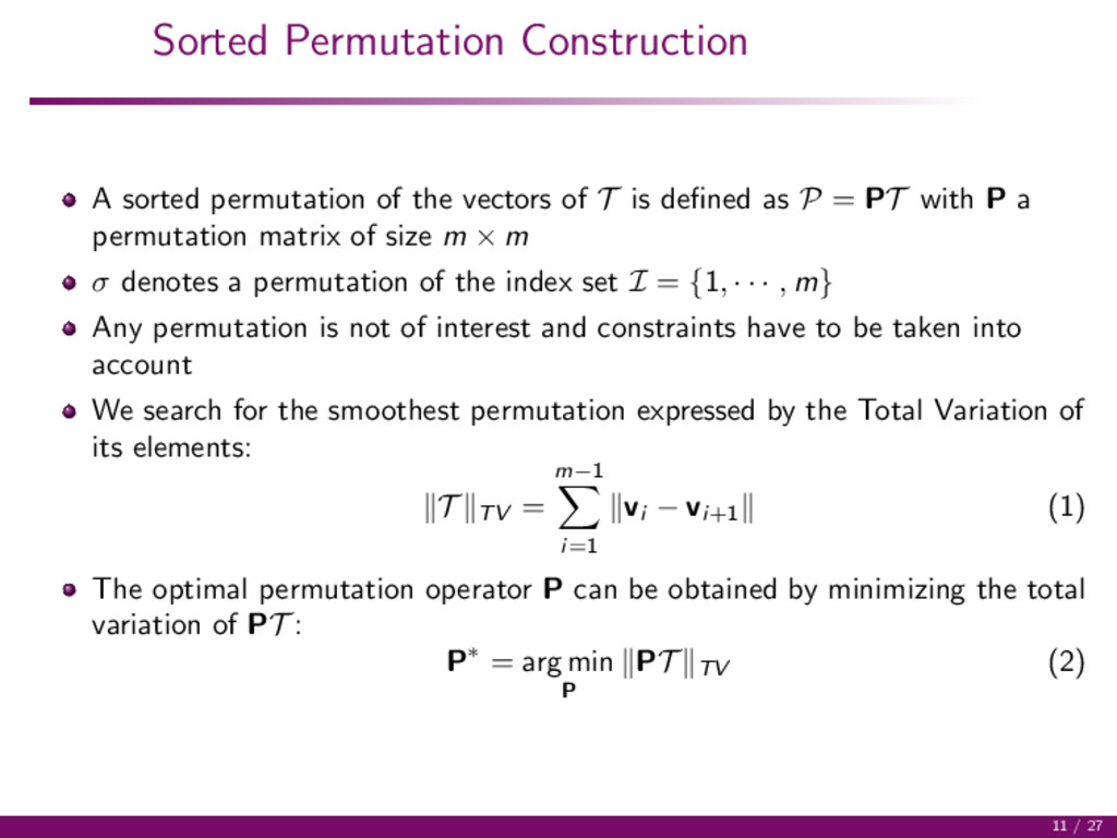
11. Sorted Permutation Construction A sorted permutation of the vectors of T is defined as P = PT with P a permutation matrix of size m × m σ denotes a permutation of the index set I = {1, · · · , m} Any permutation is not of interest and constraints have to be taken into account We search for the smoothest permutation expressed by the Total Variation of its elements: T TV = m−1 i=1 vi − vi+1 (1) The optimal permutation operator P can be obtained by minimizing the total variation of PT : P∗ = arg min P PT TV (2) 11 / 27
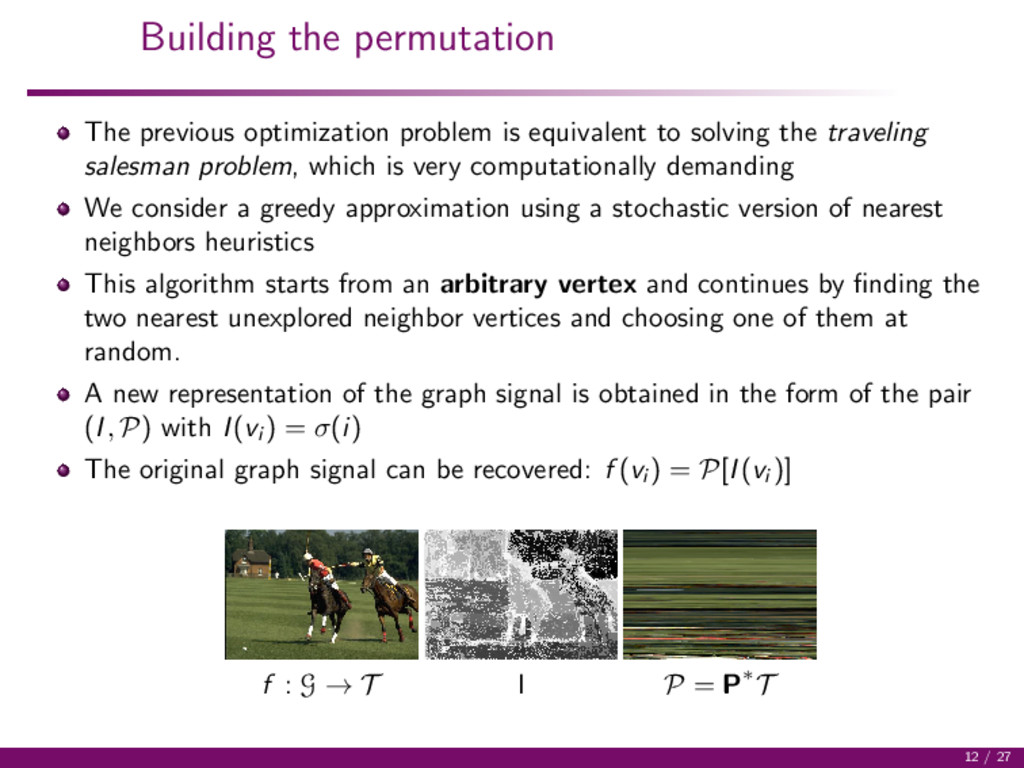
12. Building the permutation The previous optimization problem is equivalent to solving the traveling salesman problem, which is very computationally demanding We consider a greedy approximation using a stochastic version of nearest neighbors heuristics This algorithm starts from an arbitrary vertex and continues by finding the two nearest unexplored neighbor vertices and choosing one of them at random. A new representation of the graph signal is obtained in the form of the pair (I, P) with I(vi ) = σ(i) The original graph signal can be recovered: f (vi ) = P[I(vi )] f : G → T I P = P∗T 12 / 27
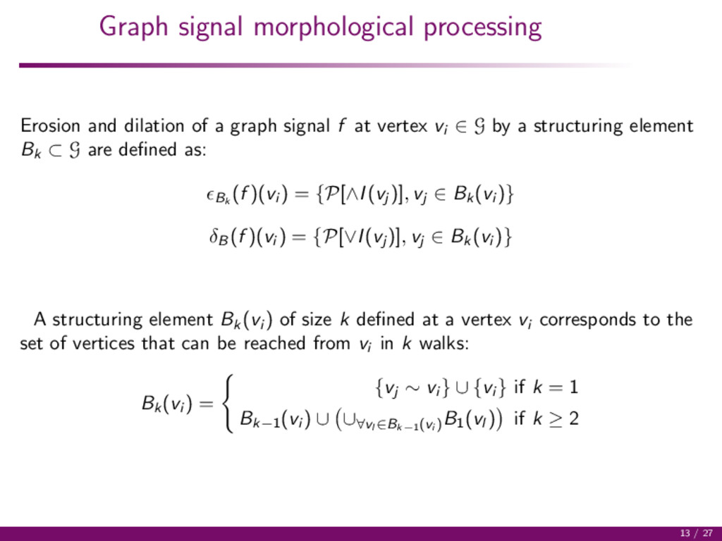
13. Graph signal morphological processing Erosion and dilation of a graph signal f at vertex vi ∈ G by a structuring element Bk ⊂ G are defined as: Bk (f )(vi ) = {P[∧I(vj )], vj ∈ Bk (vi )} δB (f )(vi ) = {P[∨I(vj )], vj ∈ Bk (vi )} A structuring element Bk (vi ) of size k defined at a vertex vi corresponds to the set of vertices that can be reached from vi in k walks: Bk (vi ) = {vj ∼ vi } ∪ {vi } if k = 1 Bk−1 (vi ) ∪ ∪∀vl ∈Bk−1(vi ) B1 (vl ) if k ≥ 2 13 / 27
14. 1 Introduction 2 One dimensional permutation ordering 3 Spectral-spatial permutation and consensus ordering 4 Results 5 Conclusion 14 / 27
15. 1 Introduction 2 One dimensional permutation ordering 3 Spectral-spatial permutation and consensus ordering 4 Results 5 Conclusion 15 / 27
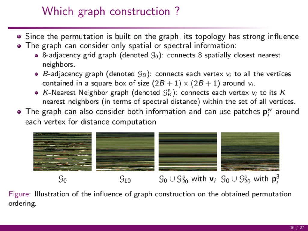
16. Which graph construction ? Since the permutation is built on the graph, its topology has strong influence The graph can consider only spatial or spectral information: 8-adjacency grid graph (denoted G0 ): connects 8 spatially closest nearest neighbors. B-adjacency graph (denoted GB ): connects each vertex vi to all the vertices contained in a square box of size (2B + 1) × (2B + 1) around vi . K-Nearest Neighbor graph (denoted Gs K ): connects each vertex vi to its K nearest neighbors (in terms of spectral distance) within the set of all vertices. The graph can also consider both information and can use patches pw i around each vertex for distance computation G0 G10 G0 ∪ Gs 20 with vi G0 ∪ Gs 20 with p3 i Figure: Illustration of the influence of graph construction on the obtained permutation ordering. 16 / 27
17. Consensus ordering The construction of the permutation starts from an arbitrary vertex Different results with different starting vertices Idea: combine several orders hi Three different aggregation strategies are considered: Instant-Runoff: determines the final order according to majority ranking votes Borda-Count: assigns each item a score Bi (vj ) = 1 − hi (vj )−1 m based on the positions and ranks the elements according to mean aggregation of the scores Weighted Borda Count: takes into account the smoothness of the order Bi s (vj ) = Bi (vj ) × ∇Pi (vj ) 17 / 27
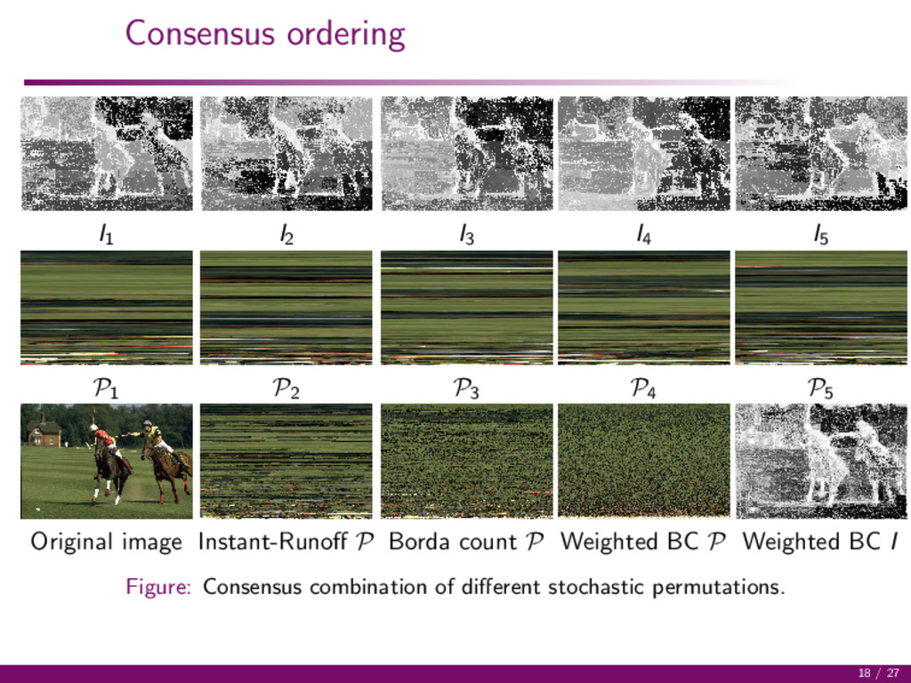
18. Consensus ordering I1 I2 I3 I4 I5 P1 P2 P3 P4 P5 Original image Instant-Runoff P Borda count P Weighted BC P Weighted BC I Figure: Consensus combination of different stochastic permutations. 18 / 27
19. 1 Introduction 2 One dimensional permutation ordering 3 Spectral-spatial permutation and consensus ordering 4 Results 5 Conclusion 19 / 27
20. 1 Introduction 2 One dimensional permutation ordering 3 Spectral-spatial permutation and consensus ordering 4 Results 5 Conclusion 20 / 27
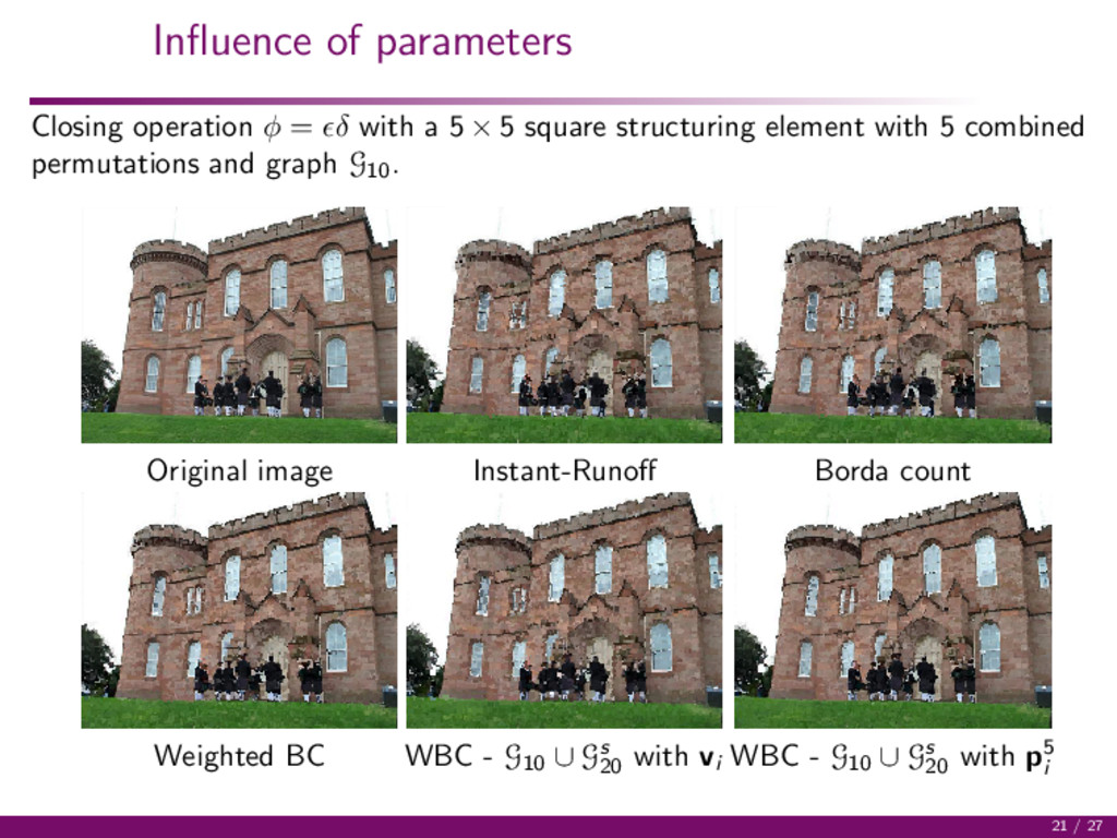
21. Influence of parameters Closing operation φ = δ with a 5 × 5 square structuring element with 5 combined permutations and graph G10 . Original image Instant-Runoff Borda count Weighted BC WBC - G10 ∪ Gs 20 with vi WBC - G10 ∪ Gs 20 with p5 i 21 / 27
22. Local versus Nonlocal Local processing based on color vectors (with a G10 graph) and a nonlocal processing based on patches (with a G10 ∪ Gs 20 graph) Original image local closing nonlocal closing 22 / 27
23. Comparison to the state-of-the-art Original image B2 δB2 δB2 − B2 Classical MM NL MM Our approach Figure: Comparison between classical MM, NL MM [Velasco-Forero, 2013], and our approach with a 5 × 5 SE. 23 / 27
24. 1 Introduction 2 One dimensional permutation ordering 3 Spectral-spatial permutation and consensus ordering 4 Results 5 Conclusion 24 / 27
25. 1 Introduction 2 One dimensional permutation ordering 3 Spectral-spatial permutation and consensus ordering 4 Results 5 Conclusion 25 / 27
26. Conclusion We have proposed: A novel approach for morphological processing of images Several stochastic orderings are constructed to obtain smooth paths on graphs The graph construction can benefit from both spatial and spectral constraints The permutation orderings are combined using weighted borda count Enables nonlocal processing 26 / 27
27. The end Publications available at : https://lezoray.users.greyc.fr 27 / 27