ISIVC 2022 Keynote

Transcript

1. MULTIVARIATE APPROACHES FOR GRAPH SIGNAL MORPHOLOGICAL PROCESSING ISIVC , El Jadida Olivier L´ EZORAY Normandie Univ, UNICAEN, ENSICAEN, CNRS, GREYC, Caen, FRANCE olivier.lezoray@unicaen.fr https://lezoray.users.greyc.fr
2. . Introduction . Complete Lattice Learning . Manifold learning for complete lattice learning . Graph signal representation . Graph signal morphological processing . Graph signal multi-layer decomposition . Stochastic permutation orderings . Stochastic Hamiltonian path . Consensus ordering . Permutation based stochastic watershed O. L´ ezoray Multivariate approaches for graph signal morphological processing / 8
3. . Introduction . Complete Lattice Learning . Manifold learning for complete lattice learning . Graph signal representation . Graph signal morphological processing . Graph signal multi-layer decomposition . Stochastic permutation orderings . Stochastic Hamiltonian path . Consensus ordering . Permutation based stochastic watershed O. L´ ezoray Multivariate approaches for graph signal morphological processing / 8
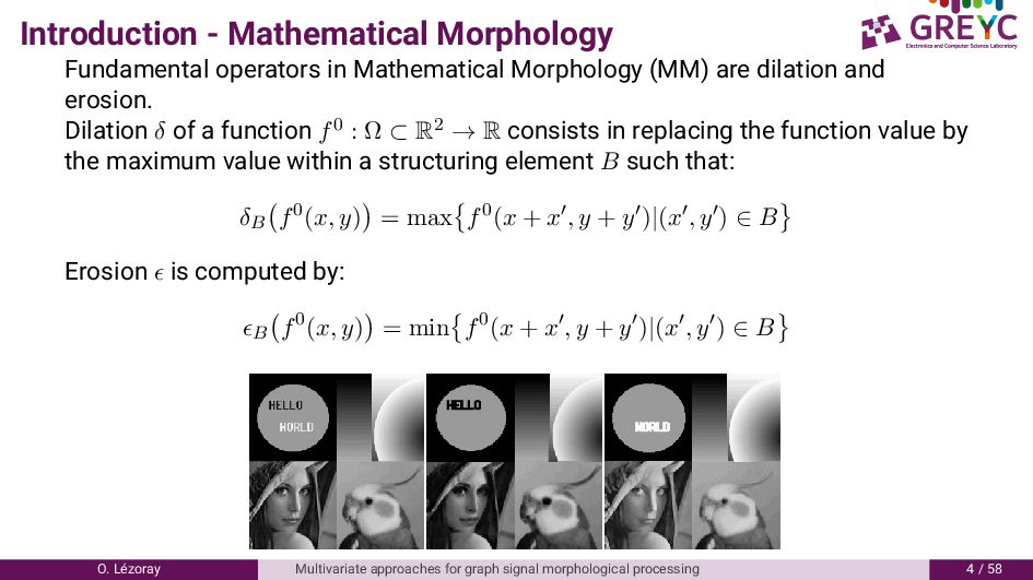
4. Introduction - Mathematical Morphology Fundamental operators in Mathematical Morphology (MM) are dilation and erosion. Dilation δ of a function f0 : Ω ⊂ R2 → R consists in replacing the function value by the maximum value within a structuring element B such that: δB f0(x, y) = max f0(x + x , y + y )|(x , y ) ∈ B Erosion is computed by: B f0(x, y) = min f0(x + x , y + y )|(x , y ) ∈ B O. L´ ezoray Multivariate approaches for graph signal morphological processing / 8
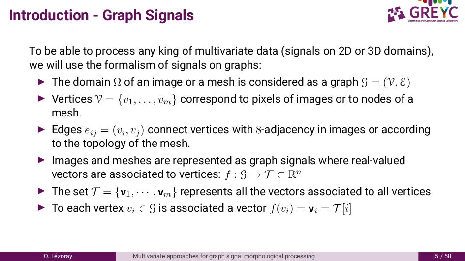
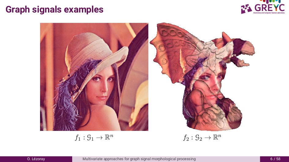
5. Introduction - Graph Signals To be able to process any king of multivariate data (signals on D or D domains), we will use the formalism of signals on graphs: The domain Ω of an image or a mesh is considered as a graph G = (V, E) Vertices V = {v1, . . . , vm} correspond to pixels of images or to nodes of a mesh. Edges eij = (vi, vj) connect vertices with 8-adjacency in images or according to the topology of the mesh. Images and meshes are represented as graph signals where real-valued vectors are associated to vertices: f : G → T ⊂ Rn The set T = {v1, · · · , vm} represents all the vectors associated to all vertices To each vertex vi ∈ G is associated a vector f(vi) = vi = T [i] O. L´ ezoray Multivariate approaches for graph signal morphological processing / 8
6. Graph signals examples f1 : G1 → Rn f2 : G2 → Rn O. L´ ezoray Multivariate approaches for graph signal morphological processing 6 / 8
7. Introduction - Complete Lattice MM needs an ordering relation within vectors: a complete lattice (T , ≤) MM is problematic for multivariate data since there is no natural ordering for vectors The framework of h-orderings can be considered for that : construct a mapping h from T to L where L is a complete lattice equipped with the conditional total ordering h : T → L and v → h(v), ∀(vi, vj) ∈ T × T vi ≤h vj ⇔ h(vi) ≤ h(vj) . ≤h denotes such an h-ordering O. L´ ezoray Multivariate approaches for graph signal morphological processing / 8
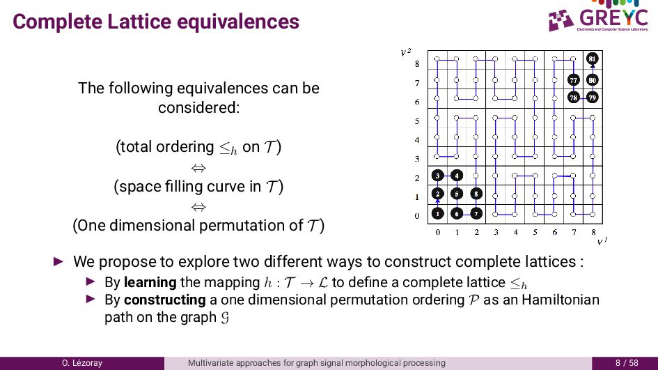
8. Complete Lattice equivalences The following equivalences can be considered: (total ordering ≤h on T ) ⇔ (space filling curve in T ) ⇔ (One dimensional permutation of T ) We propose to explore two different ways to construct complete lattices : By learning the mapping h : T → L to define a complete lattice ≤h By constructing a one dimensional permutation ordering P as an Hamiltonian path on the graph G O. L´ ezoray Multivariate approaches for graph signal morphological processing 8 / 8
9. . Introduction . Complete Lattice Learning . Manifold learning for complete lattice learning . Graph signal representation . Graph signal morphological processing . Graph signal multi-layer decomposition . Stochastic permutation orderings . Stochastic Hamiltonian path . Consensus ordering . Permutation based stochastic watershed O. L´ ezoray Multivariate approaches for graph signal morphological processing / 8
10. . Introduction . Complete Lattice Learning . Manifold learning for complete lattice learning . Graph signal representation . Graph signal morphological processing . Graph signal multi-layer decomposition . Stochastic permutation orderings . Stochastic Hamiltonian path . Consensus ordering . Permutation based stochastic watershed O. L´ ezoray Multivariate approaches for graph signal morphological processing / 8
11. Complete Lattice Learning Usual approaches to mathematical morphology define a total ordering relation using an explicit ordering: Lexicographic ordering BitMixing Ordering By proceeding this way, this is the definition of the ordering that induces the total lattice. We propose to consider the opposite. We will explicitly learn a mapping h : T → L on a multivariate graph signal. The obtained mapping will define the complete lattice in the projection space L Advantage : the learned lattice depends of the signal content and is more adaptive. h corresponds to a manifold learning operator. O. L´ ezoray Multivariate approaches for graph signal morphological processing / 8
12. Manifold-based ordering × Problem : the projection operator h cannot be linear since a distortion of the space is inevitable ! O. L´ ezoray Multivariate approaches for graph signal morphological processing / 8
13. Manifold-based ordering × Problem : the projection operator h cannot be linear since a distortion of the space is inevitable ! Solution : Consider non-linear dimensionality reduction with Laplacian Eigenmaps that corresponds to learn the manifold where the vectors live. O. L´ ezoray Multivariate approaches for graph signal morphological processing / 8
14. Manifold-based ordering × Problem : the projection operator h cannot be linear since a distortion of the space is inevitable ! Solution : Consider non-linear dimensionality reduction with Laplacian Eigenmaps that corresponds to learn the manifold where the vectors live. × Problem : Non-linear dimensionality reduction directly on the set T of vectors is not tractable in reasonable time ! O. L´ ezoray Multivariate approaches for graph signal morphological processing / 8
15. Manifold-based ordering × Problem : the projection operator h cannot be linear since a distortion of the space is inevitable ! Solution : Consider non-linear dimensionality reduction with Laplacian Eigenmaps that corresponds to learn the manifold where the vectors live. × Problem : Non-linear dimensionality reduction directly on the set T of vectors is not tractable in reasonable time ! Solution : Consider a more efficient strategy. O. L´ ezoray Multivariate approaches for graph signal morphological processing / 8
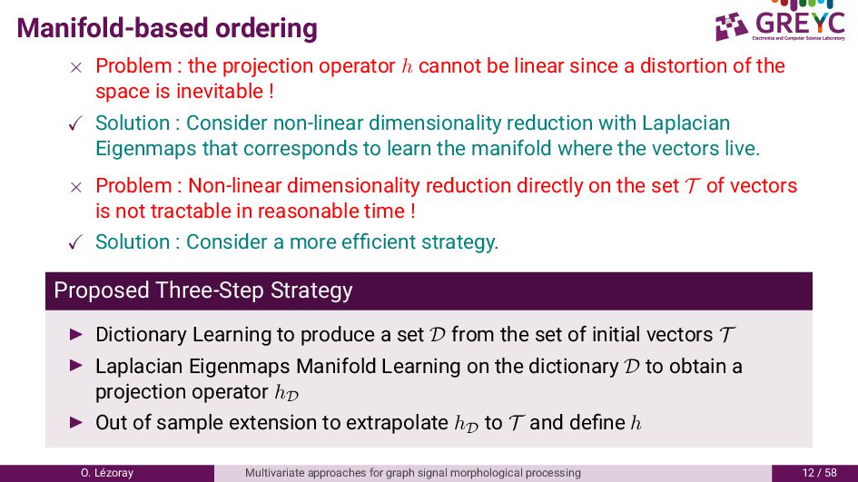
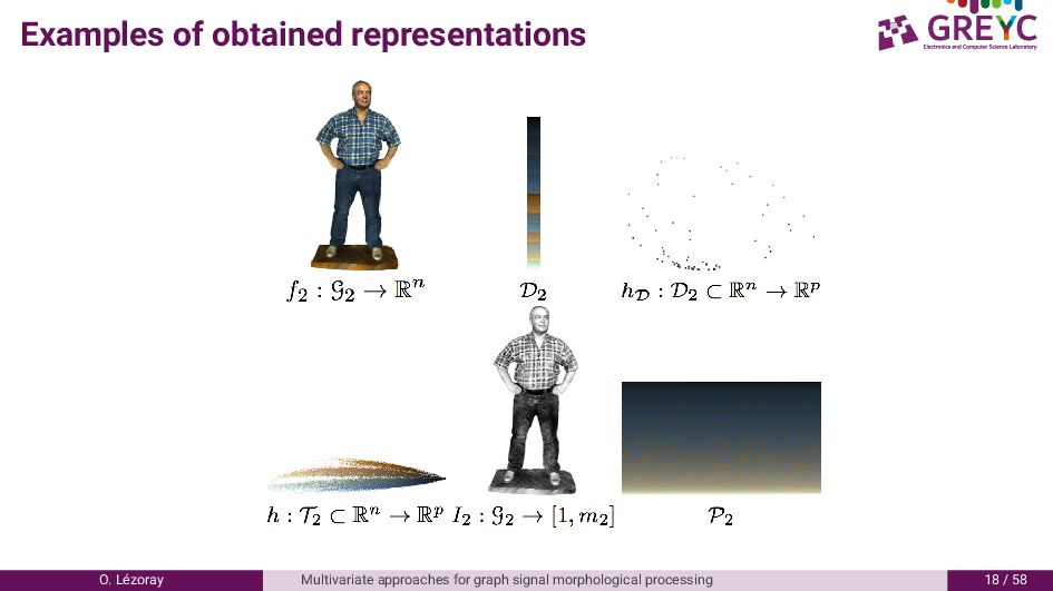
16. Manifold-based ordering × Problem : the projection operator h cannot be linear since a distortion of the space is inevitable ! Solution : Consider non-linear dimensionality reduction with Laplacian Eigenmaps that corresponds to learn the manifold where the vectors live. × Problem : Non-linear dimensionality reduction directly on the set T of vectors is not tractable in reasonable time ! Solution : Consider a more efficient strategy. Proposed Three-Step Strategy Dictionary Learning to produce a set D from the set of initial vectors T Laplacian Eigenmaps Manifold Learning on the dictionary D to obtain a projection operator hD Out of sample extension to extrapolate hD to T and define h O. L´ ezoray Multivariate approaches for graph signal morphological processing / 8
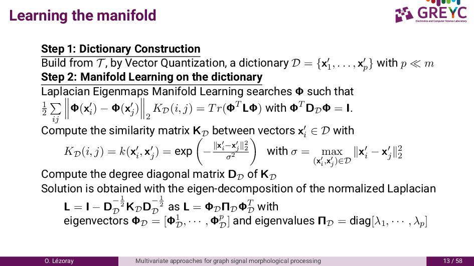
17. Learning the manifold Step : Dictionary Construction Build from T , by Vector Quantization, a dictionary D = {x1 , . . . , xp } with p m Step : Manifold Learning on the dictionary Laplacian Eigenmaps Manifold Learning searches Φ such that 1 2 ij Φ(xi ) − Φ(xj ) 2 KD(i, j) = Tr(ΦT LΦ) with ΦT DDΦ = I. Compute the similarity matrix KD between vectors xi ∈ D with KD(i, j) = k(xi , xj ) = exp − x i −x j 2 2 σ2 with σ = max (x i ,x j )∈D xi − xj 2 2 Compute the degree diagonal matrix DD of KD Solution is obtained with the eigen-decomposition of the normalized Laplacian L = I − D−1 2 D KDD−1 2 D as L = ΦDΠDΦT D with eigenvectors ΦD = [Φ1 D , · · · , Φp D ] and eigenvalues ΠD = diag[λ1, · · · , λp] O. L´ ezoray Multivariate approaches for graph signal morphological processing / 8
18. Learning the manifold A new representation hD(xi ) is obtained for each element xi of the dictionary D: hD : xi → (φ1 D (xi ), · · · , φp D (xi ))T ∈ Rp . This constructs the lattice (D, ≤hD ) with a hD -ordering, valid only on D. Step : Extrapolation of the projection ΦD to all the vectors of T Compute similarity matrices KT on T and KDT between sets D and T Compute the degree diagonal matrix DDT of KDT Extrapolate eigenvectors obtained from D to T with ˜ Φ = D−1 2 DT KT DT D−1 2 D ΦD(diag[1] − ΠD)−1 Output: The final projection h : T ⊂ R3 → L ⊂ Rp on the manifold is given by ˜ Φ and defined as h(x) = ( ˜ φ1 (x), · · · , ˜ φp (x))T . The complete lattice (T , ≤h) is obtained by using the conditional ordering on h. O. L´ ezoray Multivariate approaches for graph signal morphological processing / 8
19. . Introduction . Complete Lattice Learning . Manifold learning for complete lattice learning . Graph signal representation . Graph signal morphological processing . Graph signal multi-layer decomposition . Stochastic permutation orderings . Stochastic Hamiltonian path . Consensus ordering . Permutation based stochastic watershed O. L´ ezoray Multivariate approaches for graph signal morphological processing / 8
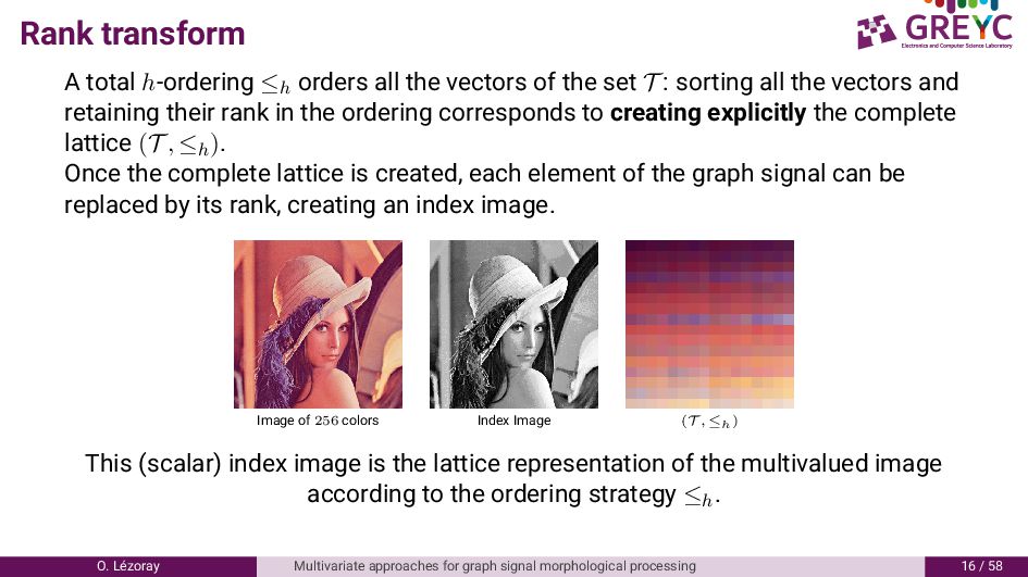
20. Rank transform A total h-ordering ≤h orders all the vectors of the set T : sorting all the vectors and retaining their rank in the ordering corresponds to creating explicitly the complete lattice (T , ≤h). Once the complete lattice is created, each element of the graph signal can be replaced by its rank, creating an index image. Image of 256 colors Index Image (T , ≤h) This (scalar) index image is the lattice representation of the multivalued image according to the ordering strategy ≤h . O. L´ ezoray Multivariate approaches for graph signal morphological processing 6 / 8
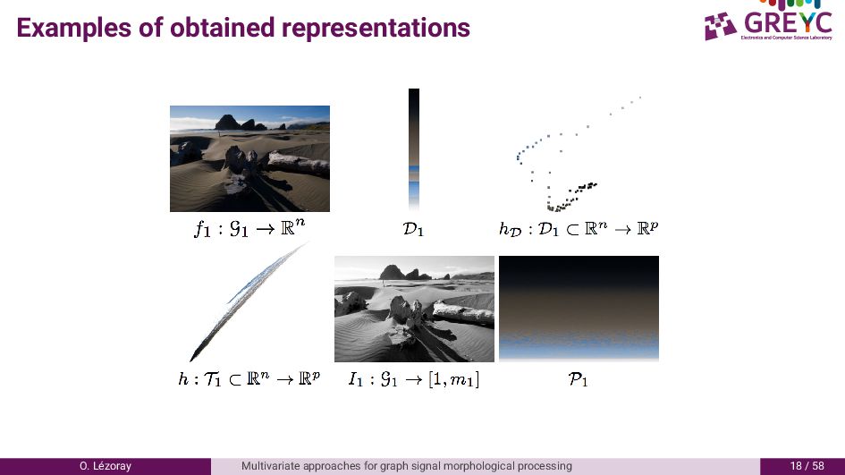
21. Graph signal representation Given the complete lattice (T , ≤h), a sorted permutation P of T is constructed P = {v1 , · · · , vm } with vi ≤h vi+1 , ∀i ∈ [1, (m − 1)]. From the ordering, an index signal I : Ω ⊂ Z2 → [1, m] is defined as: I(pi ) = {k | vk = f(pi ) = vi} . The pair (I, P) provides a new graph signal representation (the index and the palette of ordered vectors). The original signal f can be directly recovered since one has f(pi ) = P[I(pi )] = T [i] = vi O. L´ ezoray Multivariate approaches for graph signal morphological processing / 8
22. Examples of obtained representations O. L´ ezoray Multivariate approaches for graph signal morphological processing 8 / 8
23. Examples of obtained representations O. L´ ezoray Multivariate approaches for graph signal morphological processing 8 / 8
24. Comparison with the SOTA (T , ≤C ) IC : Ω → [1, m] (T , ≤CLSH ) ICLSH : Ω → [1, m] (T , ≤bm ) Ibm : Ω → [1, m] P showing (T , ≤h) I : Ω → [1, m] O. L´ ezoray Multivariate approaches for graph signal morphological processing / 8
25. From colors to patches f D hD h Color Patch Color I Color P Patch I Patch P O. L´ ezoray Multivariate approaches for graph signal morphological processing / 8
26. . Introduction . Complete Lattice Learning . Manifold learning for complete lattice learning . Graph signal representation . Graph signal morphological processing . Graph signal multi-layer decomposition . Stochastic permutation orderings . Stochastic Hamiltonian path . Consensus ordering . Permutation based stochastic watershed O. L´ ezoray Multivariate approaches for graph signal morphological processing / 8
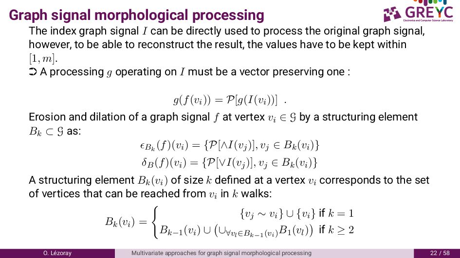
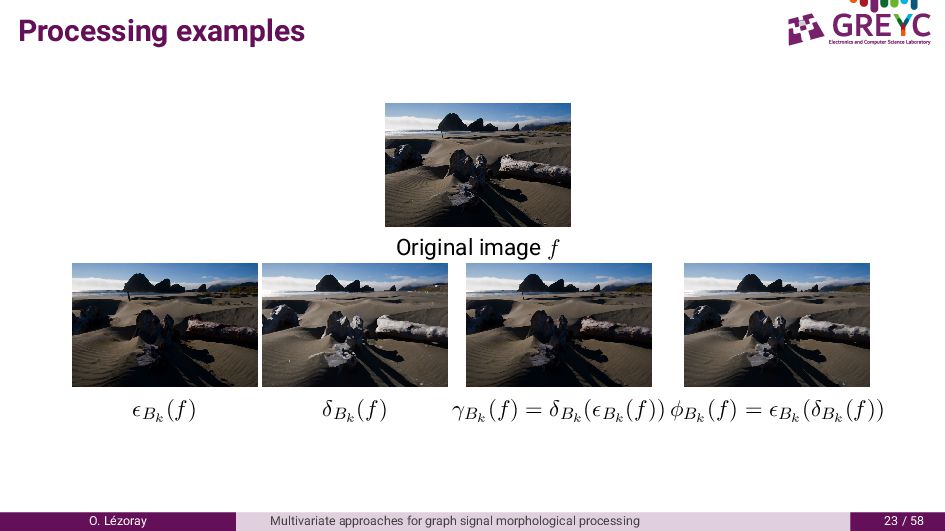
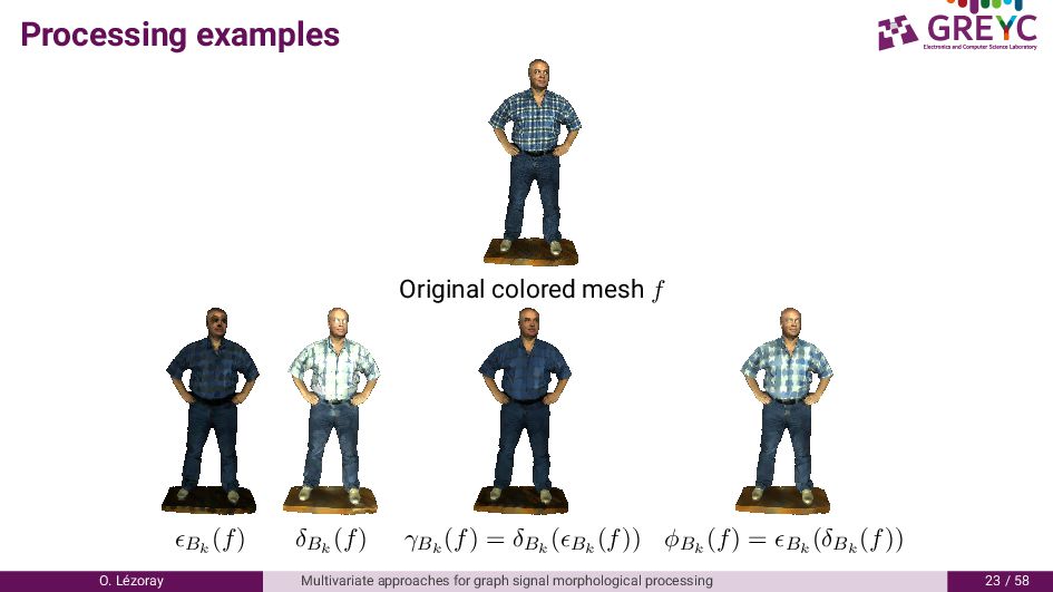
27. Graph signal morphological processing The index graph signal I can be directly used to process the original graph signal, however, to be able to reconstruct the result, the values have to be kept within [1, m]. · A processing g operating on I must be a vector preserving one : g(f(vi)) = P[g(I(vi))] . Erosion and dilation of a graph signal f at vertex vi ∈ G by a structuring element Bk ⊂ G as: Bk (f)(vi) = {P[∧I(vj)], vj ∈ Bk(vi)} δB(f)(vi) = {P[∨I(vj)], vj ∈ Bk(vi)} A structuring element Bk(vi) of size k defined at a vertex vi corresponds to the set of vertices that can be reached from vi in k walks: Bk(vi) = {vj ∼ vi} ∪ {vi} if k = 1 Bk−1(vi) ∪ ∪∀vl∈Bk−1(vi) B1(vl) if k ≥ 2 O. L´ ezoray Multivariate approaches for graph signal morphological processing / 8
28. Processing examples Original image f Bk (f) δBk (f) γBk (f) = δBk ( Bk (f)) φBk (f) = Bk (δBk (f)) O. L´ ezoray Multivariate approaches for graph signal morphological processing / 8
29. Processing examples Original colored mesh f Bk (f) δBk (f) γBk (f) = δBk ( Bk (f)) φBk (f) = Bk (δBk (f)) O. L´ ezoray Multivariate approaches for graph signal morphological processing / 8
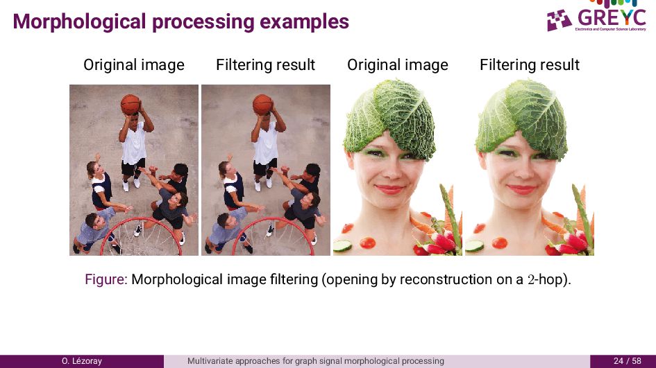
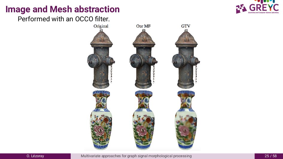
30. Morphological processing examples Original image Filtering result Original image Filtering result Figure: Morphological image filtering (opening by reconstruction on a 2-hop). O. L´ ezoray Multivariate approaches for graph signal morphological processing / 8
31. Image and Mesh abstraction Performed with an OCCO filter. O. L´ ezoray Multivariate approaches for graph signal morphological processing / 8
32. Image and Mesh abstraction Performed with an OCCO filter. O. L´ ezoray Multivariate approaches for graph signal morphological processing / 8
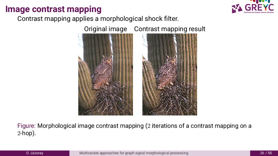
33. Image contrast mapping Contrast mapping applies a morphological shock filter. Original image Contrast mapping result Figure: Morphological image contrast mapping (2 iterations of a contrast mapping on a 2-hop). O. L´ ezoray Multivariate approaches for graph signal morphological processing 6 / 8
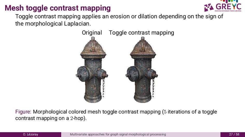
34. Mesh toggle contrast mapping Toggle contrast mapping applies an erosion or dilation depending on the sign of the morphological Laplacian. Original Toggle contrast mapping Figure: Morphological colored mesh toggle contrast mapping (5 iterations of a toggle contrast mapping on a 2-hop). O. L´ ezoray Multivariate approaches for graph signal morphological processing / 8
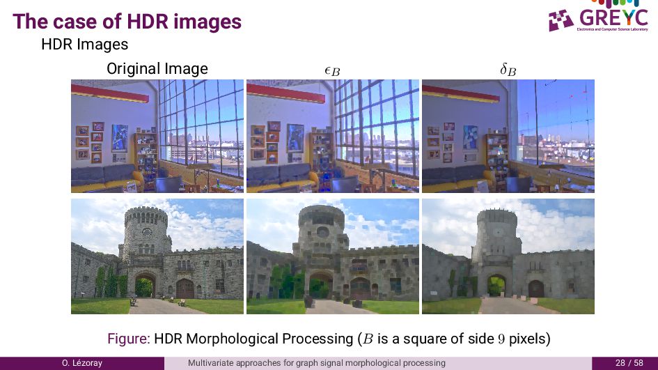
35. The case of HDR images HDR Images Original Image B δB Figure: HDR Morphological Processing (B is a square of side 9 pixels) O. L´ ezoray Multivariate approaches for graph signal morphological processing 8 / 8
36. Morphological Tone Mapping Durand & Dorsey MM Tone Mapping O. L´ ezoray Multivariate approaches for graph signal morphological processing / 8
37. . Introduction . Complete Lattice Learning . Manifold learning for complete lattice learning . Graph signal representation . Graph signal morphological processing . Graph signal multi-layer decomposition . Stochastic permutation orderings . Stochastic Hamiltonian path . Consensus ordering . Permutation based stochastic watershed O. L´ ezoray Multivariate approaches for graph signal morphological processing / 8
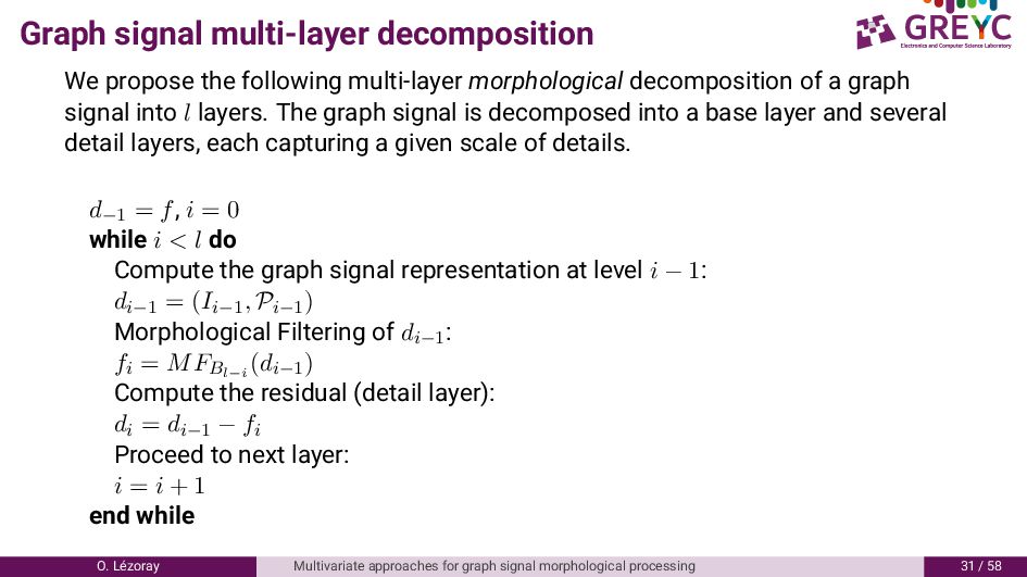
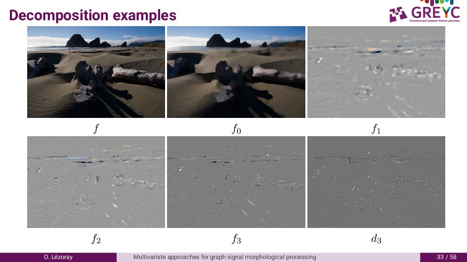
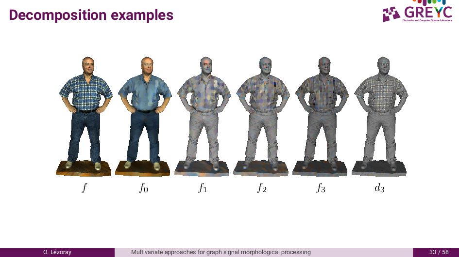
38. Graph signal multi-layer decomposition We propose the following multi-layer morphological decomposition of a graph signal into l layers. The graph signal is decomposed into a base layer and several detail layers, each capturing a given scale of details. d−1 = f, i = 0 while i < l do Compute the graph signal representation at level i − 1: di−1 = (Ii−1, Pi−1) Morphological Filtering of di−1 : fi = MFBl−i (di−1) Compute the residual (detail layer): di = di−1 − fi Proceed to next layer: i = i + 1 end while O. L´ ezoray Multivariate approaches for graph signal morphological processing / 8
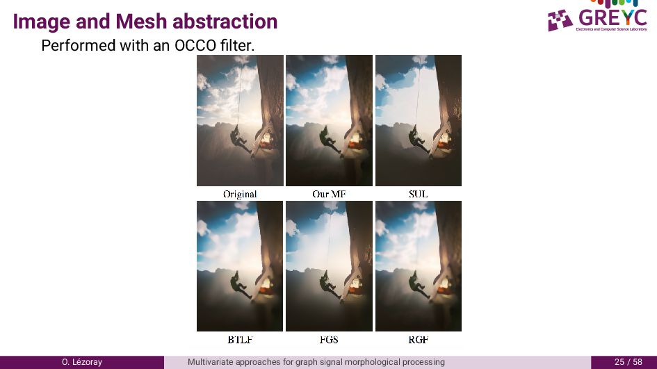
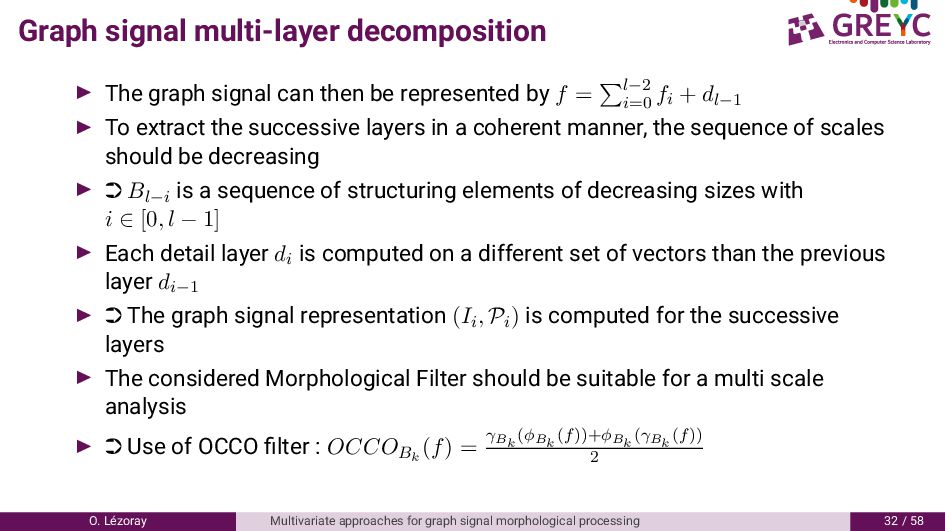
39. Graph signal multi-layer decomposition The graph signal can then be represented by f = l−2 i=0 fi + dl−1 To extract the successive layers in a coherent manner, the sequence of scales should be decreasing · Bl−i is a sequence of structuring elements of decreasing sizes with i ∈ [0, l − 1] Each detail layer di is computed on a different set of vectors than the previous layer di−1 · The graph signal representation (Ii, Pi) is computed for the successive layers The considered Morphological Filter should be suitable for a multi scale analysis · Use of OCCO filter : OCCOBk (f) = γBk (φBk (f))+φBk (γBk (f)) 2 O. L´ ezoray Multivariate approaches for graph signal morphological processing / 8
40. Decomposition examples f f0 f1 f2 f3 d3 O. L´ ezoray Multivariate approaches for graph signal morphological processing / 8
41. Decomposition examples f f0 f1 f2 f3 d3 O. L´ ezoray Multivariate approaches for graph signal morphological processing / 8
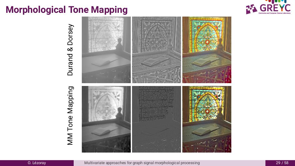
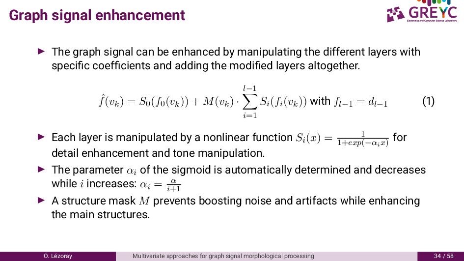
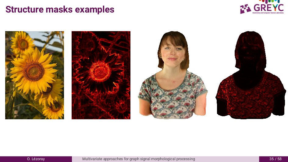
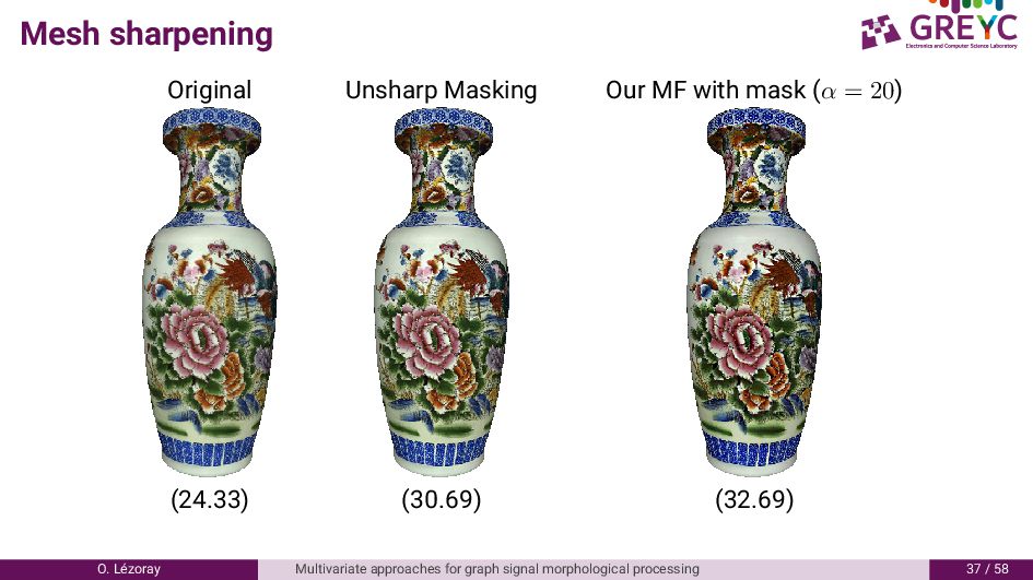
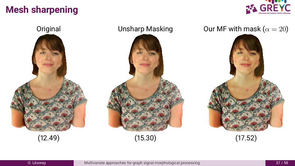
42. Graph signal enhancement The graph signal can be enhanced by manipulating the different layers with specific coefficients and adding the modified layers altogether. ˆ f(vk) = S0(f0(vk)) + M(vk) · l−1 i=1 Si(fi(vk)) with fl−1 = dl−1 ( ) Each layer is manipulated by a nonlinear function Si(x) = 1 1+exp(−αix) for detail enhancement and tone manipulation. The parameter αi of the sigmoid is automatically determined and decreases while i increases: αi = α i+1 A structure mask M prevents boosting noise and artifacts while enhancing the main structures. O. L´ ezoray Multivariate approaches for graph signal morphological processing / 8
43. Structure masks examples O. L´ ezoray Multivariate approaches for graph signal morphological processing / 8
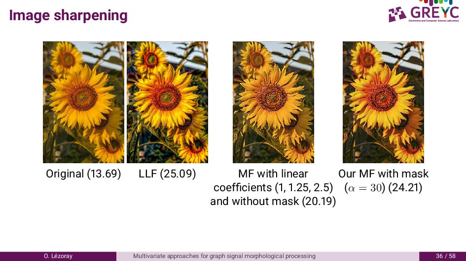
44. Image sharpening Original ( .6 ) LLF ( . ) MF with linear Our MF with mask coefficients ( , . , . ) (α = 30) ( . ) and without mask ( . ) O. L´ ezoray Multivariate approaches for graph signal morphological processing 6 / 8
45. Mesh sharpening Original Unsharp Masking Our MF with mask (α = 20) ( . ) ( .6 ) ( .6 ) O. L´ ezoray Multivariate approaches for graph signal morphological processing / 8
46. Mesh sharpening Original Unsharp Masking Our MF with mask (α = 20) ( . ) ( . ) ( . ) O. L´ ezoray Multivariate approaches for graph signal morphological processing / 8
47. . Introduction . Complete Lattice Learning . Manifold learning for complete lattice learning . Graph signal representation . Graph signal morphological processing . Graph signal multi-layer decomposition . Stochastic permutation orderings . Stochastic Hamiltonian path . Consensus ordering . Permutation based stochastic watershed O. L´ ezoray Multivariate approaches for graph signal morphological processing 8 / 8
48. . Introduction . Complete Lattice Learning . Manifold learning for complete lattice learning . Graph signal representation . Graph signal morphological processing . Graph signal multi-layer decomposition . Stochastic permutation orderings . Stochastic Hamiltonian path . Consensus ordering . Permutation based stochastic watershed O. L´ ezoray Multivariate approaches for graph signal morphological processing / 8
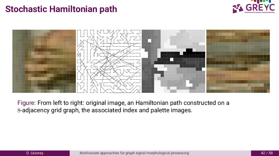
49. Stochastic Hamiltonian path Our proposal : construct a complete lattice with an image-adaptive h-ordering based on an space filling curve on the graph · an Hamiltonian path Equivalent as defining a sorted permutation of the vectors of T It is defined as P = PT with P a permutation matrix of size m × m Any permutation is not of interest, we search for the smoothest permutation expressed by the Total Variation of its elements: T TV = m−1 i=1 vi − vi+1 The optimal permutation operator P∗ can be obtained by minimizing the total variation of PT : P∗ = arg min P PT TV O. L´ ezoray Multivariate approaches for graph signal morphological processing / 8
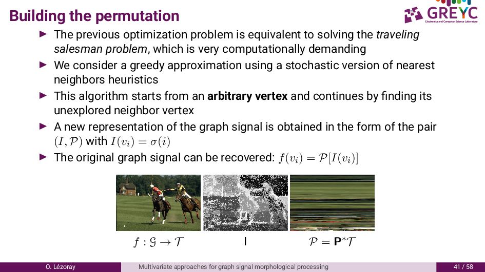
50. Building the permutation The previous optimization problem is equivalent to solving the traveling salesman problem, which is very computationally demanding We consider a greedy approximation using a stochastic version of nearest neighbors heuristics This algorithm starts from an arbitrary vertex and continues by finding its unexplored neighbor vertex A new representation of the graph signal is obtained in the form of the pair (I, P) with I(vi) = σ(i) The original graph signal can be recovered: f(vi) = P[I(vi)] f : G → T I P = P∗T O. L´ ezoray Multivariate approaches for graph signal morphological processing / 8
51. Stochastic Hamiltonian path 0 1 20 21 2 3 22 23 4 5 24 25 6 26 27 7 8 28 9 10 30 29 11 367 12 13 31 32 14 15 136 55 16 17 37 18 19 39 40 41 42 43 375 45 47 50 52 33 34 54 53 35 36 38 59 60 44 63 64 46 66 67 48 49 69 70 51 71 74 75 56 57 76 58 77 79 80 61 81 82 62 120 259 83 65 85 86 68 87 88 89 91 72 73 93 94 95 78 100 101 103 84 104 165 99 108 90 111 92 96 97 116 117 98 224 102 121 123 105 124 106 125 127 107 110 109 189 112 113 114 115 118 119 139 161 122 142 143 144 126 145 128 129 130 131 132 133 152 134 153 154 135 155 156 285 137 138 249 140 160 366 141 162 163 164 146 166 167 147 148 149 150 170 151 171 284 157 158 159 179 182 183 184 168 169 188 172 173 174 175 176 177 178 180 181 200 241 201 203 185 186 204 207 187 206 324 190 209 210 191 192 213 193 194 214 195 196 197 198 199 218 202 221 222 205 208 211 212 232 215 216 237 217 266 219 239 220 240 223 242 245 225 226 394 246 227 228 248 229 230 231 250 233 234 235 236 257 238 258 261 260 262 243 244 263 264 247 354 270 251 271 272 252 253 273 254 274 275 255 256 276 334 280 282 281 283 265 286 267 287 288 268 269 293 294 277 278 279 299 300 301 302 303 304 289 290 311 291 292 310 295 296 315 297 298 316 321 323 305 306 326 307 308 309 312 331 333 313 314 332 317 318 319 339 320 340 341 322 342 343 325 344 346 327 347 328 329 348 330 352 353 355 335 336 356 357 337 338 360 361 363 345 364 368 349 350 371 351 372 376 358 359 377 379 380 362 382 383 384 365 385 386 387 389 369 370 388 391 373 374 395 396 378 397 399 398 381 390 392 393 Figure: From left to right: original image, an Hamiltonian path constructed on a 8-adjacency grid graph, the associated index and palette images. O. L´ ezoray Multivariate approaches for graph signal morphological processing / 8
52. Stochastic nature of the ordering Original image I1 P1 I2 P2 δ γ φ O. L´ ezoray Multivariate approaches for graph signal morphological processing / 8
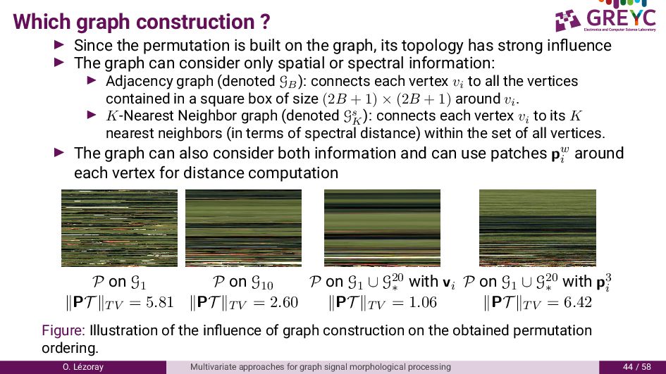
53. Which graph construction ? Since the permutation is built on the graph, its topology has strong influence The graph can consider only spatial or spectral information: Adjacency graph (denoted GB ): connects each vertex vi to all the vertices contained in a square box of size (2B + 1) × (2B + 1) around vi . K-Nearest Neighbor graph (denoted Gs K ): connects each vertex vi to its K nearest neighbors (in terms of spectral distance) within the set of all vertices. The graph can also consider both information and can use patches pw i around each vertex for distance computation P on G1 P on G10 P on G1 ∪ G20 ∗ with vi P on G1 ∪ G20 ∗ with p3 i PT TV = 5.81 PT TV = 2.60 PT TV = 1.06 PT TV = 6.42 Figure: Illustration of the influence of graph construction on the obtained permutation ordering. O. L´ ezoray Multivariate approaches for graph signal morphological processing / 8
54. . Introduction . Complete Lattice Learning . Manifold learning for complete lattice learning . Graph signal representation . Graph signal morphological processing . Graph signal multi-layer decomposition . Stochastic permutation orderings . Stochastic Hamiltonian path . Consensus ordering . Permutation based stochastic watershed O. L´ ezoray Multivariate approaches for graph signal morphological processing / 8
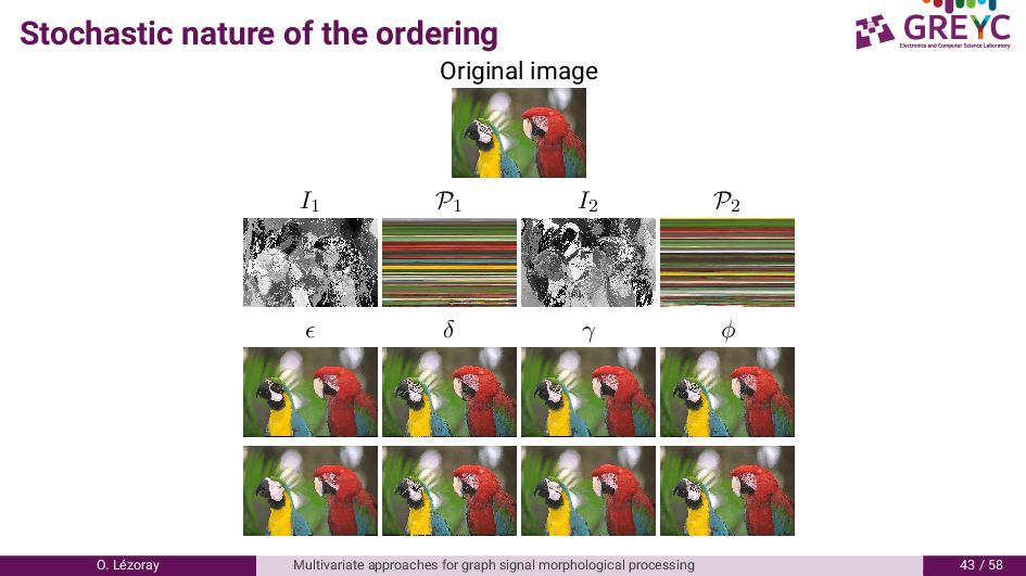
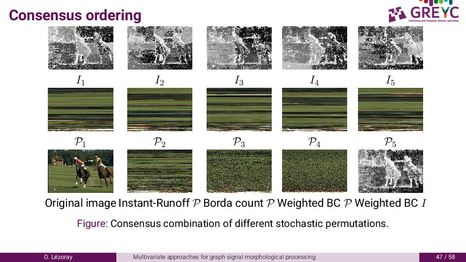
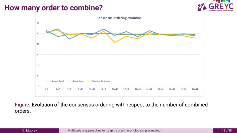
55. Consensus ordering The construction of the permutation starts from an arbitrary vertex Different results with different starting vertices Idea: combine several orders hi Three different aggregation strategies are considered: Instant-Runoff: determines the final order according to majority ranking votes Borda-Count: assigns each item a score Bi(vj) = 1 − hi(vj)−1 m based on the positions and ranks the elements according to mean aggregation of the scores Weighted Borda Count: takes into account the smoothness of the order Bi s (vj) = Bi(vj) × ∇Pi(vj) O. L´ ezoray Multivariate approaches for graph signal morphological processing 6 / 8
56. Consensus ordering I1 I2 I3 I4 I5 P1 P2 P3 P4 P5 Original image Instant-Runoff P Borda count P Weighted BC P Weighted BC I Figure: Consensus combination of different stochastic permutations. O. L´ ezoray Multivariate approaches for graph signal morphological processing / 8
57. How many order to combine? 0 10 20 30 40 50 60 3vs5 5vs7 7vs9 9vs11 11vs13 13vs15 15vs17 17vs19 19vs21 21vs23 23vs25 25vs27 27vs29 29vs31 Consensus ordering evolution Instant-Runoff Borda Count Weighted Borda Count Figure: Evolution of the consensus ordering with respect to the number of combined orders. O. L´ ezoray Multivariate approaches for graph signal morphological processing 8 / 8
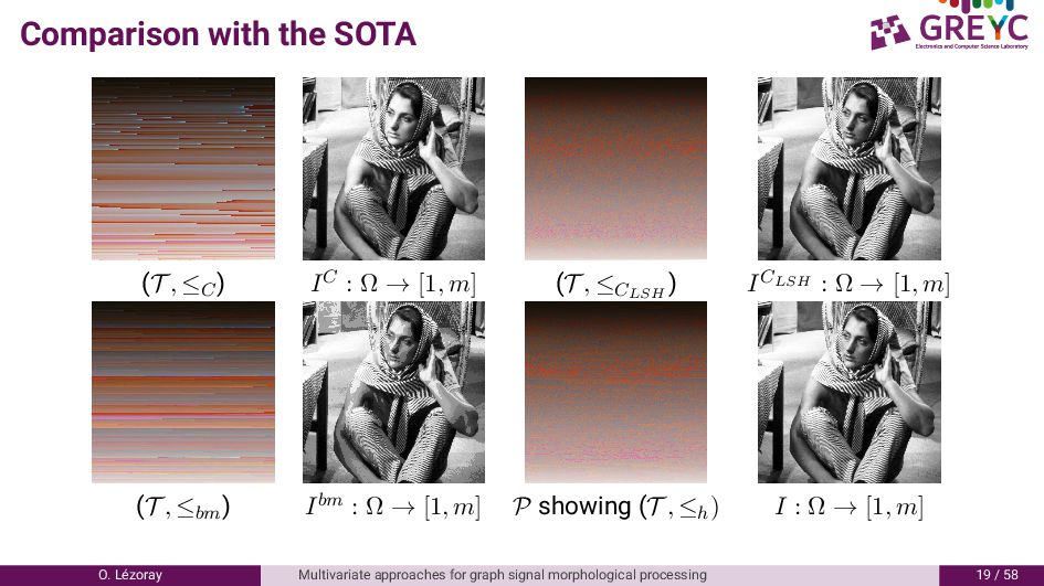
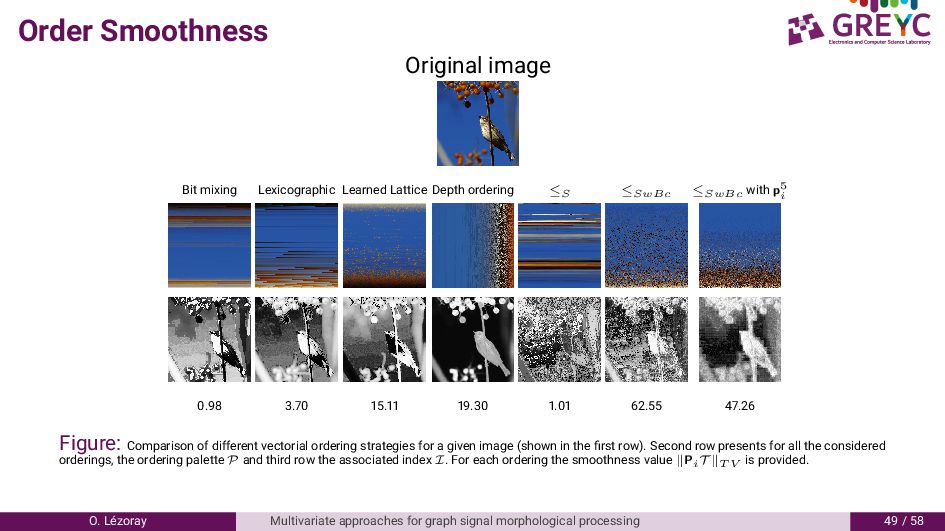
58. Order Smoothness Original image Bit mixing Lexicographic Learned Lattice Depth ordering ≤S ≤SwBc ≤SwBc with p5 i . 8 . . . . 6 . . 6 Figure: Comparison of different vectorial ordering strategies for a given image (shown in the first row). Second row presents for all the considered orderings, the ordering palette P and third row the associated index I. For each ordering the smoothness value PiT T V is provided. O. L´ ezoray Multivariate approaches for graph signal morphological processing / 8
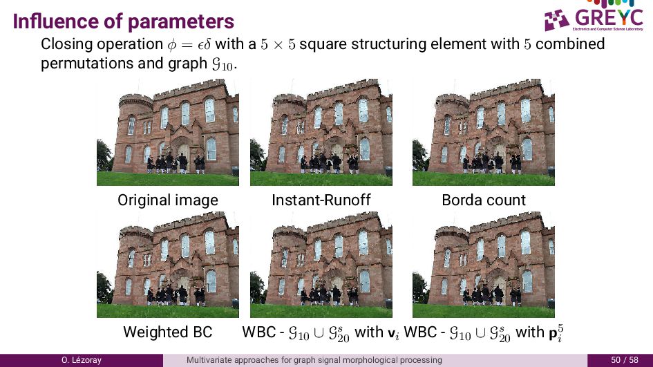
59. Influence of parameters Closing operation φ = δ with a 5 × 5 square structuring element with 5 combined permutations and graph G10 . Original image Instant-Runoff Borda count Weighted BC WBC - G10 ∪ Gs 20 with vi WBC - G10 ∪ Gs 20 with p5 i O. L´ ezoray Multivariate approaches for graph signal morphological processing / 8
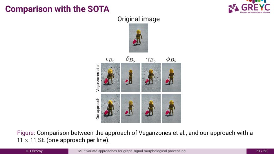
60. Comparison with the SOTA Original image B5 δB5 γB5 φB5 Veganzones et al. Our approach Figure: Comparison between the approach of Veganzones et al., and our approach with a 11 × 11 SE (one approach per line). O. L´ ezoray Multivariate approaches for graph signal morphological processing / 8
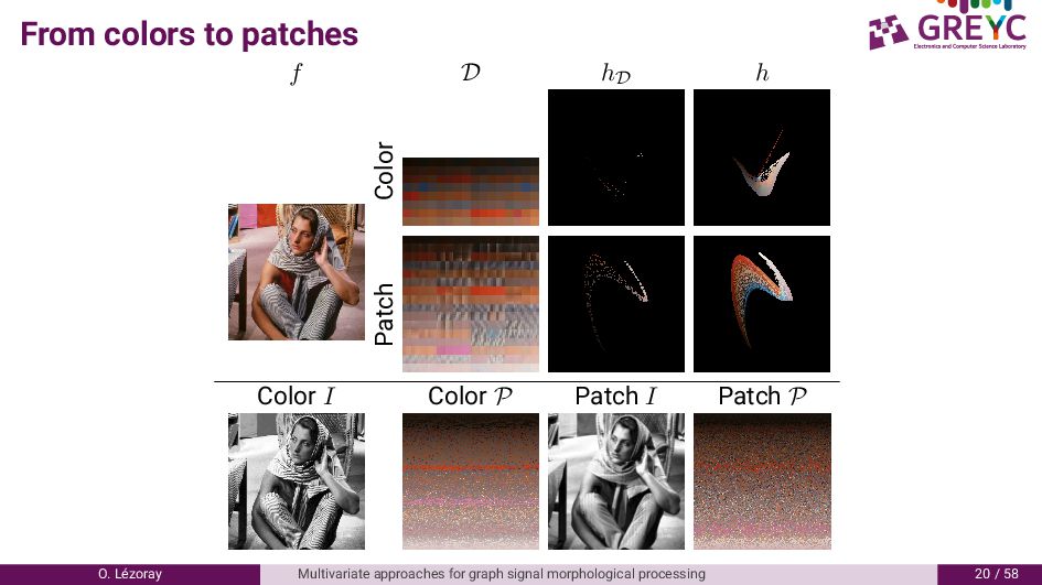
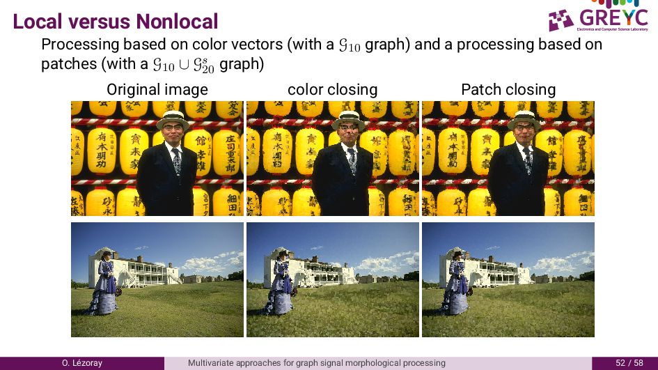
61. Local versus Nonlocal Processing based on color vectors (with a G10 graph) and a processing based on patches (with a G10 ∪ Gs 20 graph) Original image color closing Patch closing O. L´ ezoray Multivariate approaches for graph signal morphological processing / 8
62. . Introduction . Complete Lattice Learning . Manifold learning for complete lattice learning . Graph signal representation . Graph signal morphological processing . Graph signal multi-layer decomposition . Stochastic permutation orderings . Stochastic Hamiltonian path . Consensus ordering . Permutation based stochastic watershed O. L´ ezoray Multivariate approaches for graph signal morphological processing / 8
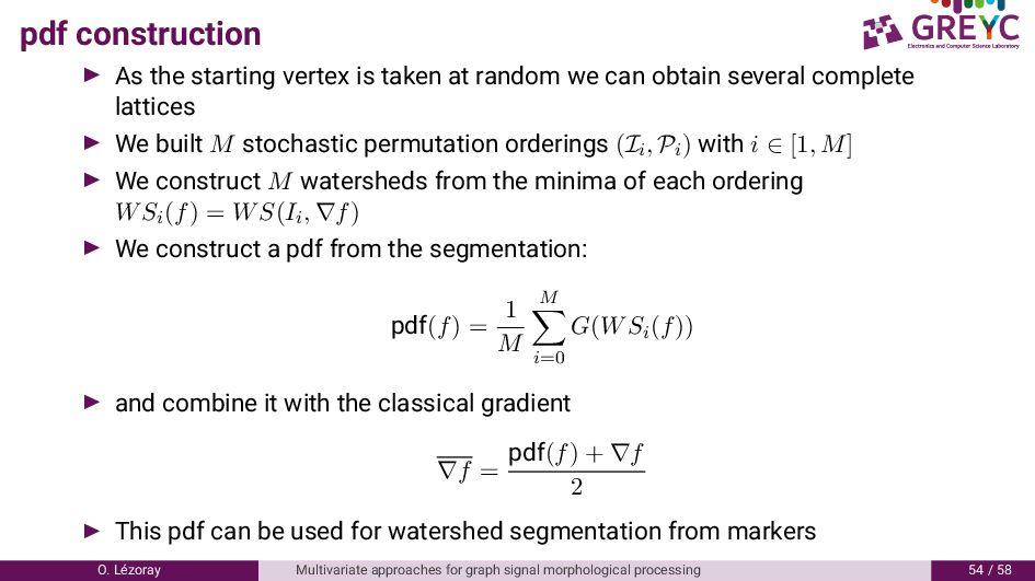
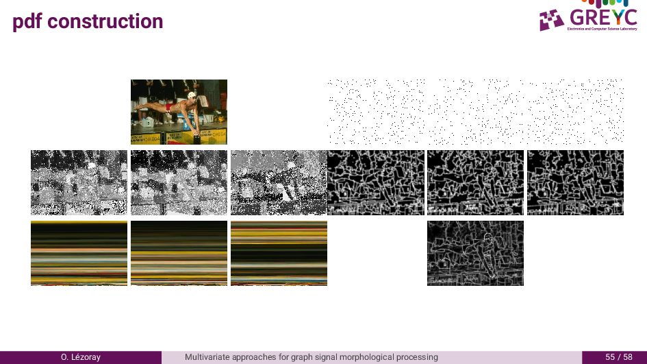
63. pdf construction As the starting vertex is taken at random we can obtain several complete lattices We built M stochastic permutation orderings (Ii, Pi) with i ∈ [1, M] We construct M watersheds from the minima of each ordering WSi(f) = WS(Ii, ∇f) We construct a pdf from the segmentation: pdf(f) = 1 M M i=0 G(WSi(f)) and combine it with the classical gradient ∇f = pdf(f) + ∇f 2 This pdf can be used for watershed segmentation from markers O. L´ ezoray Multivariate approaches for graph signal morphological processing / 8
64. pdf construction O. L´ ezoray Multivariate approaches for graph signal morphological processing / 8
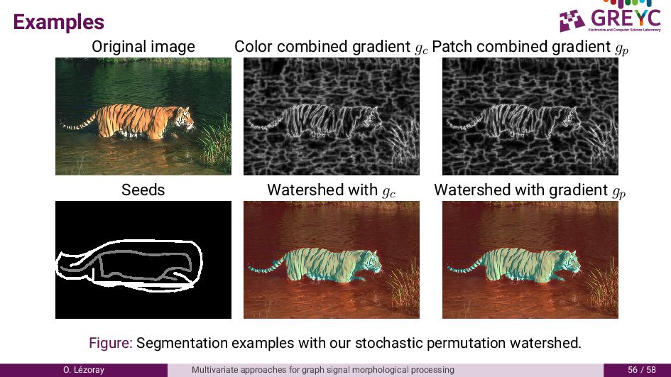
65. Examples Original image Color combined gradient gc Patch combined gradient gp Seeds Watershed with gc Watershed with gradient gp Figure: Segmentation examples with our stochastic permutation watershed. O. L´ ezoray Multivariate approaches for graph signal morphological processing 6 / 8
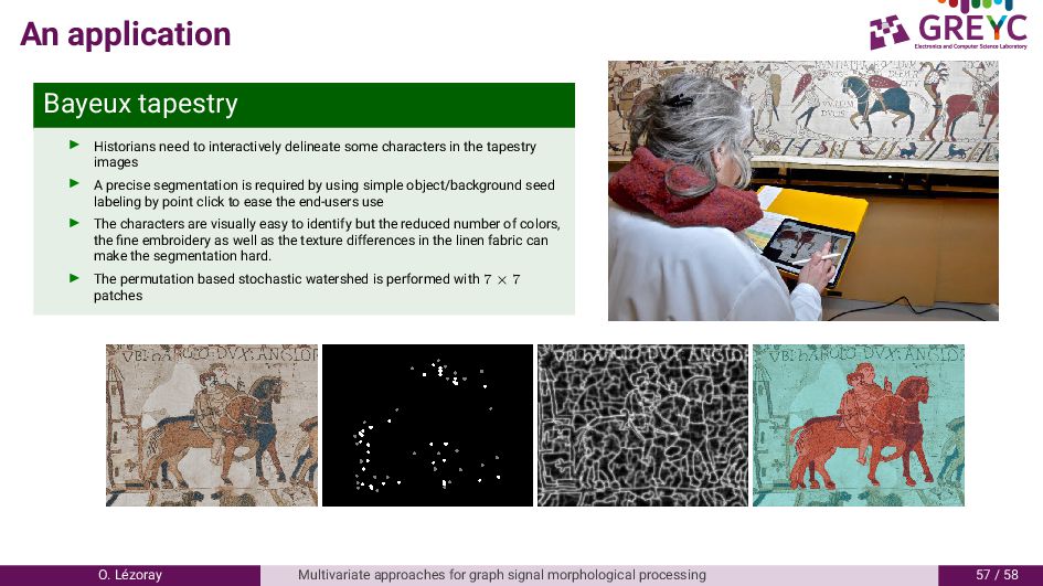
66. An application Bayeux tapestry Historians need to interactively delineate some characters in the tapestry images A precise segmentation is required by using simple object/background seed labeling by point click to ease the end-users use The characters are visually easy to identify but the reduced number of colors, the fine embroidery as well as the texture differences in the linen fabric can make the segmentation hard. The permutation based stochastic watershed is performed with 7 × 7 patches O. L´ ezoray Multivariate approaches for graph signal morphological processing / 8
67. The end [thank you] Any Questions ? olivier.lezoray@unicaen.fr https://lezoray.users.greyc.fr O. L´ ezoray Multivariate approaches for graph signal morphological processing 8 / 8