p-Laplacian regularization of signals on directed graphs

Transcript

1. p-Laplacian regularization of signals on directed graphs Zeina Abu-Aisheh, S´ ebastien Bougleux and Olivier L´ ezoray Normandie Univ, UNICAEN, ENSICAEN, CNRS, GREYC, 14000 Caen, France olivier.lezoray@unicaen.fr https://lezoray.users.greyc.fr
2. 1 Introduction and Motivations 2 Contribution: p-Laplacian on Directed Graph Signals 3 Experiments and Results 4 Conclusions and Perspectives 2 / 32
3. 1 Introduction and Motivations 2 Contribution: p-Laplacian on Directed Graph Signals 3 Experiments and Results 4 Conclusions and Perspectives 3 / 32
4. Graphs are appealing tools Structured data can be represented by graph signals (f : V → Rn) 4 / 32
5. Graphs Signal Processing (GSP) Extending the classical discrete signal processing tools to signals living on an underlying irregular graph Applications: (To cite a few) Neuroimaging: [Ktena17] Social network analysis: [Bruna17, Schlichtkrull17] Computer graphics: [Wang17, Simonovsky17] GeoScience: [Bayram17] 5 / 32
6. Undirected Graphs Signals Definition of Undirected Graph Signals G = (V, E) V is a set of vertices E ⊆ V × V is a set of edges vi ∈ V is the ith vertex eij = {vi , vj } is the edge between vi and vj w : E → R+. w(vi , vj ) = 0 if eij ∈ E and 0 otherwise. d(vi ) = eij ∈E wij is the degree of vi 6 / 32
7. Undirected Graphs Signals Definition of Undirected Graph Signals G = (V, E) V is a set of vertices E ⊆ V × V is a set of edges vi ∈ V is the ith vertex eij = {vi , vj } is the edge between vi and vj w : E → R+. w(vi , vj ) = 0 if eij ∈ E and 0 otherwise. d(vi ) = eij ∈E wij is the degree of vi v1 v2 v3 v4 v5
8. Undirected Graphs Signals Definition of Undirected Graph Signals G = (V, E) V is a set of vertices E ⊆ V × V is a set of edges vi ∈ V is the ith vertex eij = {vi , vj } is the edge between vi and vj w : E → R+. w(vi , vj ) = 0 if eij ∈ E and 0 otherwise. d(vi ) = eij ∈E wij is the degree of vi v1 v2 v3 v4 v5 e14 e15 e 24 e23 e53 6 / 32
9. Directed Graphs Signals Definition of Directed Graph Signals G = (V, E) V is a set of vertices E ⊆ V × V is a set of edges vi ∈ V is the ith vertex vj → vi is the edge from vj and vi w : E → R+. w(vi , vj ) = 0 if vi → vj ∈ E and 0 otherwise. (vj → vi = vi → vj ) d+ (vi ) = vi →vj ∈E wij is the out-degree of vi d− (vi ) = vi ←vj ∈E wji is the in-degree of vi v1 v2 v3 v4 v5
10. Directed Graphs Signals Definition of Directed Graph Signals G = (V, E) V is a set of vertices E ⊆ V × V is a set of edges vi ∈ V is the ith vertex vj → vi is the edge from vj and vi w : E → R+. w(vi , vj ) = 0 if vi → vj ∈ E and 0 otherwise. (vj → vi = vi → vj ) d+ (vi ) = vi →vj ∈E wij is the out-degree of vi d− (vi ) = vi ←vj ∈E wji is the in-degree of vi v1 v2 v3 v4 v5 v1 → v4 v1 → v5 v 2 → v 4 v2 → v3 v5 → v3 7 / 32
11. Laplacians on Undirected Graph Signals One of the main ingredients of GSP 8 / 32
12. Laplacians on Undirected Graph Signals One of the main ingredients of GSP A notion of frequency for graph signals (Fourier-like transform) 8 / 32
13. Laplacians on Undirected Graph Signals One of the main ingredients of GSP A notion of frequency for graph signals (Fourier-like transform) Famous laplacians for undirected graphs [Luxburg07] (matrix form): 8 / 32
14. Laplacians on Undirected Graph Signals One of the main ingredients of GSP A notion of frequency for graph signals (Fourier-like transform) Famous laplacians for undirected graphs [Luxburg07] (matrix form): The Combinatorial Laplacian: L = D − W 8 / 32
15. Laplacians on Undirected Graph Signals One of the main ingredients of GSP A notion of frequency for graph signals (Fourier-like transform) Famous laplacians for undirected graphs [Luxburg07] (matrix form): The Combinatorial Laplacian: L = D − W The Normalized Laplacian: ˜ L = D−1/2LD−1/2 = I − D−1/2WD−1/2 8 / 32
16. Laplacians on Undirected Graph Signals One of the main ingredients of GSP A notion of frequency for graph signals (Fourier-like transform) Famous laplacians for undirected graphs [Luxburg07] (matrix form): The Combinatorial Laplacian: L = D − W The Normalized Laplacian: ˜ L = D−1/2LD−1/2 = I − D−1/2WD−1/2 The random walk Laplacian: Lrw = D−1L = I − D−1W 8 / 32
17. Laplacians on Undirected Graph Signals One of the main ingredients of GSP A notion of frequency for graph signals (Fourier-like transform) Famous laplacians for undirected graphs [Luxburg07] (matrix form): The Combinatorial Laplacian: L = D − W The Normalized Laplacian: ˜ L = D−1/2LD−1/2 = I − D−1/2WD−1/2 The random walk Laplacian: Lrw = D−1L = I − D−1W But: This does not concerns the nonlinear extension of the Laplacian: the p-Laplacian The definition of p-laplacians has not been generalized for directed graphs 8 / 32
18. Laplacians on Undirected Graph Signals One of the main ingredients of GSP A notion of frequency for graph signals (Fourier-like transform) Famous laplacians for undirected graphs [Luxburg07] (matrix form): The Combinatorial Laplacian: L = D − W The Normalized Laplacian: ˜ L = D−1/2LD−1/2 = I − D−1/2WD−1/2 The random walk Laplacian: Lrw = D−1L = I − D−1W But: This does not concerns the nonlinear extension of the Laplacian: the p-Laplacian The definition of p-laplacians has not been generalized for directed graphs Thus: we address the general case of p-Laplacians on directed graphs 8 / 32
19. 1 Introduction and Motivations 2 Contribution: p-Laplacian on Directed Graph Signals 3 Experiments and Results 4 Conclusions and Perspectives 9 / 32
20. p-Laplacian on Directed Graphs Notations H(V): The Hilbert space of real-valued functions defined on V H(E): The Hilbert space of real-valued functions defined on E f : V → Rn of H(V) is a graph signal Mapping each vi to a vector f(vi ). H(V) is endowed with the inner product f , h H(V) = vi ∈V f (vi )h(vi ). f , h : V → R are two functions of H(V) H(E) is endowed with the inner product F, H H(E) = eij ∈E F(eij )H(eij ) F, H : E → R are two functions of H(E) 10 / 32
21. p-Laplacian on Directed Graphs (1) Ingredients Directed difference operator dw : H(V) → H(E) (dw f )(vi , vj ) is the directed operator on vi → vj Adjoint operator d∗ w : H(E) → H(V) expressed at a vertex vi ∈ V as: Obtained from the inner products since H, dw f H(E) = d∗ w H, f H(V) . The gradient operator of a function at vertex vi ∈ V: (∇w f)(vi ) = ((dw f )(vi , vj ))T , ∀(vi → vj ) ∈ E Lp norm of the gradient: (∇w f)(vi ) p = vi →vj ∈E |(dw f )(vi , vj )|p 1/p 11 / 32
22. p-Laplacian on Directed Graphs (2) Definition: p-Laplacian the p-Laplacian ∆p w f : H(V) → H(V) can be formulated as the discrete analogue of the continuous one defined in [Elmoataz2008]: ∆p w f (vi ) = 1 2 d∗ w ∇w f(vi ) p−2 2 (dw f )(vi , vj ) = 1 2 d∗ w (dw f )(vi , vj ) ∇w f(vi ) 2−p 2 where p ∈ (0, +∞). Previous works only considered symmetric undirected graphs with (dw f )(vi , vj ) on undirected edges. 12 / 32
23. Proposal: Three p-Laplacian on Directed Graphs p-Laplacian ∆p w f (vi ) = 1 2 d∗ w ∇w f(vi ) p−2 2 (dw f )(vi , vj ) = 1 2 d∗ w (dw f )(vi , vj ) ∇w f(vi ) 2−p 2 Proposal: Three p-Laplacian on Directed Graphs The Combinatorial directed p-laplacian (∆p w ): (dw f )(vi , vj ) = w(vi , vj )(f (vj ) − f (vi )) (d∗ w H)(vi ) = vj →vi H(vj , vi )w(vj , vi ) − vi →vj H(vi , vj )w(vi , vj ) . The normalized combinatorial directed p-laplacian ( ˜ ∆p w ): (dw f )(vi , vj ) = w(vi , vj ) f (vj ) d−(vj ) − f (vi ) √ d+(vi ) (d∗ w H)(vi ) = vj →vi H(vj ,vi )w(vj ,vi ) √ d−(vi ) − vi →vj H(vi ,vj )w(vi ,vj ) √ d+(vi ) . 13 / 32
24. Proposal: Three p-Laplacian on Directed Graphs p-Laplacian ∆p w f (vi ) = 1 2 d∗ w ∇w f(vi ) p−2 2 (dw f )(vi , vj ) = 1 2 d∗ w (dw f )(vi , vj ) ∇w f(vi ) 2−p 2 Proposal: Three p-Laplacian operators The random-walk directed p-laplacian (∆p,rw w ): (dw f )(vi , vj ) = w(vi ,vj ) √ d+(vi ) (f (vj ) − f (vi )) (d∗ w H)(vi ) = vj →vi H(vj ,vi )w(vj ,vi ) √ d+(vi ) − vi →vj H(vi ,vj )w(vi ,vj ) √ d+(vi ) . 14 / 32
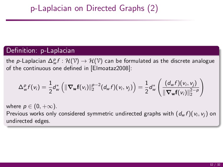
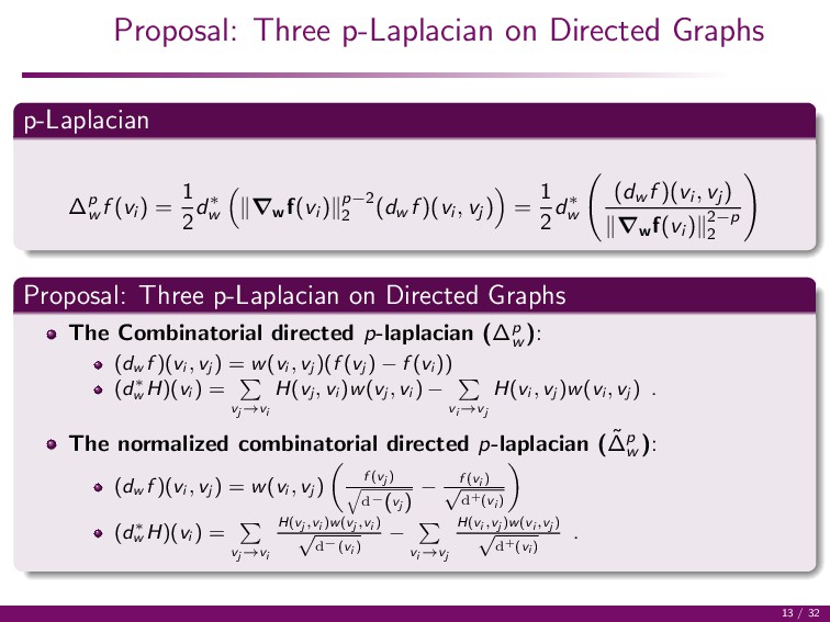
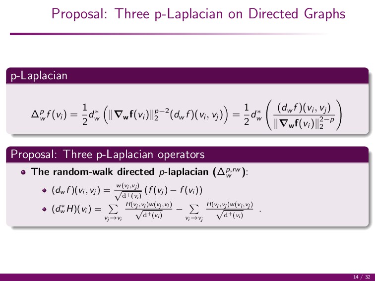
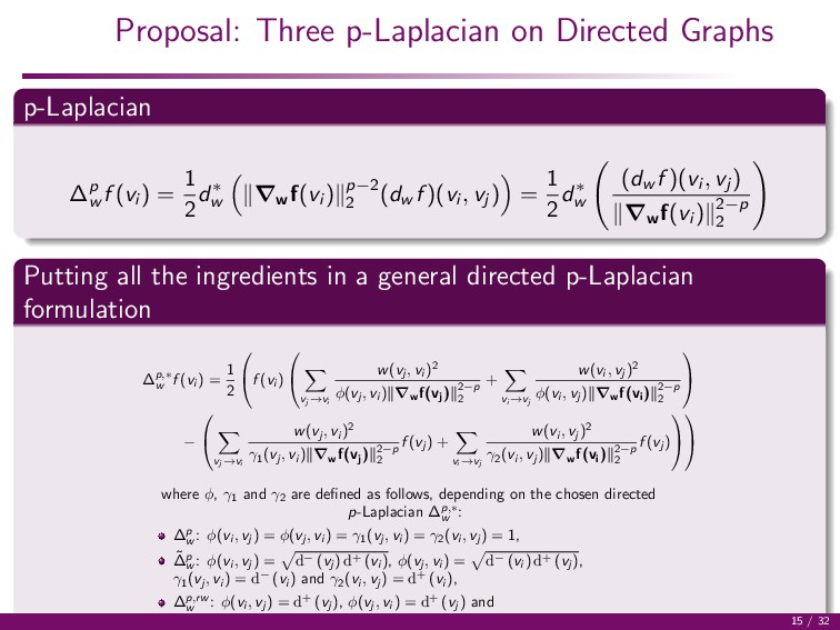
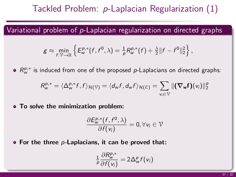
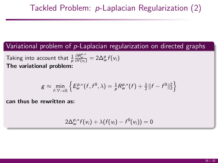
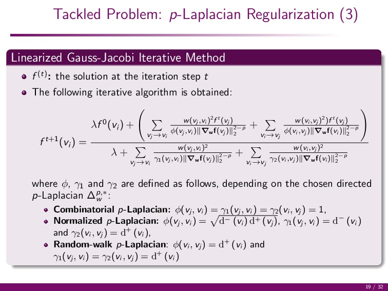
25. Proposal: Three p-Laplacian on Directed Graphs p-Laplacian ∆p w f (vi ) = 1 2 d∗ w ∇w f(vi ) p−2 2 (dw f )(vi , vj ) = 1 2 d∗ w (dw f )(vi , vj ) ∇w f(vi ) 2−p 2 Putting all the ingredients in a general directed p-Laplacian formulation ∆p,∗ w f (vi ) = 1 2  f (vi )   vj →vi w(vj , vi )2 φ(vj , vi ) ∇w f(vj ) 2−p 2 + vi →vj w(vi , vj )2 φ(vi , vj ) ∇w f(vi ) 2−p 2   −   vj →vi w(vj , vi )2 γ1 (vj , vi ) ∇w f(vj ) 2−p 2 f (vj ) + vi →vj w(vi , vj )2 γ2 (vi , vj ) ∇w f(vi ) 2−p 2 f (vj )     where φ, γ1 and γ2 are defined as follows, depending on the chosen directed p-Laplacian ∆p,∗ w : ∆p w : φ(vi , vj ) = φ(vj , vi ) = γ1 (vj , vi ) = γ2 (vi , vj ) = 1, ˜ ∆p w : φ(vi , vj ) = d− (vj ) d+ (vi ), φ(vj , vi ) = d− (vi ) d+ (vj ), γ1 (vj , vi ) = d− (vi ) and γ2 (vi , vj ) = d+ (vi ), ∆p,rw w : φ(vi , vj ) = d+ (vj ), φ(vj , vi ) = d+ (vj ) and γ1 (vj , vi ) = γ2 (vi , vj ) = d+ (vi ). 15 / 32
26. Tackled Problem: p-Laplacian Regularization p-Laplacian Regularization on Directed Graphs Variational problem of p-Laplacian regularization on directed graphs: g ≈ min f :V→R Ep,∗ w (f , f 0, λ) = 1 p Rp,∗ w (f ) + λ 2 f − f 0 2 2 Energy: Ep,∗ w Regularization functional: Rp,∗ w (f ) Approximation term: λ 2 f − f 0 2 2 Noisy graph signal: f 0 : V → Rn f 0 = g + n: where g is the clean graph corrupted by a given noise n How to recover the uncorrupted function g? Solution: Find f : V → Rn which is regular enough on G and close enough to f 0 16 / 32
27. Tackled Problem: p-Laplacian Regularization (1) Variational problem of p-Laplacian regularization on directed graphs g ≈ min f :V→R Ep,∗ w (f , f 0, λ) = 1 p Rp,∗ w (f ) + λ 2 f − f 0 2 2 , Rp,∗ w is induced from one of the proposed p-Laplacians on directed graphs: Rp,∗ w = ∆p,∗ w f , f H(V) = dw f , dw f H(E) = vi ∈V (∇w f)(vi ) p 2 To solve the minimization problem: ∂Ep,∗ w (f , f 0, λ) ∂f (vi ) = 0, ∀vi ∈ V For the three p-Laplacians, it can be proved that: 1 p ∂Rp,∗ w ∂f (vi ) = 2∆p w f (vi ) 17 / 32
28. Tackled Problem: p-Laplacian Regularization (2) Variational problem of p-Laplacian regularization on directed graphs Taking into account that 1 p ∂Rp,∗ w ∂f (vi ) = 2∆p w f (vi ) The variational problem: g ≈ min f :V→R Ep,∗ w (f , f 0, λ) = 1 p Rp,∗ w (f ) + λ 2 f − f 0 2 2 can thus be rewritten as: 2∆p,∗ w f (vi ) + λ(f (vi ) − f 0(vi )) = 0 18 / 32
29. Tackled Problem: p-Laplacian Regularization (3) Linearized Gauss-Jacobi Iterative Method f (t): the solution at the iteration step t The following iterative algorithm is obtained: f t+1(vi ) = λf 0(vi ) + vj →vi w(vj ,vi )2f t (vj ) φ(vj ,vi ) ∇wf(vj ) 2−p 2 + vi →vj w(vi ,vj )2)f t (vj ) φ(vi ,vj ) ∇wf(vi ) 2−p 2 λ + vj →vi w(vj ,vi )2 γ1(vj ,vi ) ∇wf(vj ) 2−p 2 + vi →vj w(vi ,vj )2 γ2(vi ,vj ) ∇wf(vi ) 2−p 2 where φ, γ1 and γ2 are defined as follows, depending on the chosen directed p-Laplacian ∆p,∗ w : Combinatorial p-Laplacian: φ(vj , vi ) = γ1 (vj , vi ) = γ2 (vi , vj ) = 1, Normalized p-Laplacian: φ(vj , vi ) = d− (vi ) d+ (vj ), γ1 (vj , vi ) = d− (vi ) and γ2 (vi , vj ) = d+ (vi ), Random-walk p-Laplacian: φ(vi , vj ) = d+ (vi ) and γ1 (vj , vi ) = γ2 (vi , vj ) = d+ (vi ) 19 / 32
30. 1 Introduction and Motivations 2 Contribution: p-Laplacian on Directed Graph Signals 3 Experiments and Results 4 Conclusions and Perspectives 20 / 32
31. Experiments and Results General Protocol PSNR values is used to compare the filtering results 21 / 32
32. Experiments and Results General Protocol PSNR values is used to compare the filtering results To weight the edges of the graphs: w(vi , vj ) = 1 − Ff0 τ (vi )−Ff0 τ (vj ) 2 max vk →vl ∈E Ff0 τ (vk )−Ff0 τ (vl ) 2 21 / 32
33. Experiments and Results General Protocol PSNR values is used to compare the filtering results To weight the edges of the graphs: w(vi , vj ) = 1 − Ff0 τ (vi )−Ff0 τ (vj ) 2 max vk →vl ∈E Ff0 τ (vk )−Ff0 τ (vl ) 2 Ff0 τ (vi ) = f 0(vj ) : vj ∈ Nτ (vi ) ∪ {vi } T corresponds to the set of values around vi within a τ-hop Nτ (vi ) 21 / 32
34. Experiments and Results General Protocol PSNR values is used to compare the filtering results To weight the edges of the graphs: w(vi , vj ) = 1 − Ff0 τ (vi )−Ff0 τ (vj ) 2 max vk →vl ∈E Ff0 τ (vk )−Ff0 τ (vl ) 2 Ff0 τ (vi ) = f 0(vj ) : vj ∈ Nτ (vi ) ∪ {vi } T corresponds to the set of values around vi within a τ-hop Nτ (vi ) Two types of graphs are considered: 21 / 32
35. Experiments and Results General Protocol PSNR values is used to compare the filtering results To weight the edges of the graphs: w(vi , vj ) = 1 − Ff0 τ (vi )−Ff0 τ (vj ) 2 max vk →vl ∈E Ff0 τ (vk )−Ff0 τ (vl ) 2 Ff0 τ (vi ) = f 0(vj ) : vj ∈ Nτ (vi ) ∪ {vi } T corresponds to the set of values around vi within a τ-hop Nτ (vi ) Two types of graphs are considered: 8-adjacency directed grid graph (G0 ) Connecting each vertex to its 8 spatially closest nearest neighbors 21 / 32
36. Experiments and Results General Protocol PSNR values is used to compare the filtering results To weight the edges of the graphs: w(vi , vj ) = 1 − Ff0 τ (vi )−Ff0 τ (vj ) 2 max vk →vl ∈E Ff0 τ (vk )−Ff0 τ (vl ) 2 Ff0 τ (vi ) = f 0(vj ) : vj ∈ Nτ (vi ) ∪ {vi } T corresponds to the set of values around vi within a τ-hop Nτ (vi ) Two types of graphs are considered: 8-adjacency directed grid graph (G0 ) Connecting each vertex to its 8 spatially closest nearest neighbors k-nearest neighbor directed graphs (Gα,τ k ) Connecting each vertex to its k nearest neighbors in terms of Ff0 τ L2 norm within a α-hop) 21 / 32
37. Protocol for 2D color Images Images corrupted by Gaussian noise 22 / 32
38. Protocol for 2D color Images Images corrupted by Gaussian noise G0 : 8-adjacency directed grid graph (with λ = 0.05, p=1) 22 / 32
39. Protocol for 2D color Images Images corrupted by Gaussian noise G0 : 8-adjacency directed grid graph (with λ = 0.05, p=1) G0 ∪ G5,1 10 : 8-adjacency directed grid graph augmented with a 10-nearest neighbor graph within a 5-hop (λ = 0.09 with patches of size 3 × 3) 22 / 32
40. Results for Filtering 2D color Images Original Image Corrupted image (σ = 15): 24.69dB ∆p w ˜ ∆p w ∆p,rw w p = 1, G0 26.47dB 28.79dB 29.33dB p = 1, G0 ∪ G5,1 10 28.15dB 27.11dB 30.12dB Figure: 23 / 32
41. Protocol for Image Database Images corrupted by Gaussian noise 24 / 32
42. Protocol for Image Database Images corrupted by Gaussian noise f : V → R28×28 24 / 32
43. Protocol for Image Database Images corrupted by Gaussian noise f : V → R28×28 Selection of a subset of 90 images from the MNIST database for digits 0, 1, 3 24 / 32
44. Protocol for Image Database Images corrupted by Gaussian noise f : V → R28×28 Selection of a subset of 90 images from the MNIST database for digits 0, 1, 3 G∞,0 5 : A 5-nearest neighbor graph on the whole dataset ( α = ∞) 24 / 32
45. Protocol for Image Database Images corrupted by Gaussian noise f : V → R28×28 Selection of a subset of 90 images from the MNIST database for digits 0, 1, 3 G∞,0 5 : A 5-nearest neighbor graph on the whole dataset ( α = ∞) λ = 10−4 24 / 32
46. Results for Filtering an Image Database Original DB Corrupted DB (σ = 40) G∞,0 5 Filtered DB Figure: p-Laplacian regularization of a corrupted image database (with ˜ ∆p w , p = 1, and λ = 10−4). 25 / 32
47. Results for Filtering an Image Database (1) σ 20 40 ∆p,∗ w ∆p w ˜ ∆p w ∆p,rw w ∆p w ˜ ∆p w ∆p,rw w p = 2 14.54 14.63 14.56 12.91 13.08 12.88 p = 1 16.37 16.83 16.80 14.01 13.11 13.73 Table: Image database regularization on directed graphs (λ = 10−4). Best results (in terms of PSNR) are bold faced. 26 / 32
48. Protocol for 3D Colored Meshes The meshes are 3D scans from an ancient building and a person 27 / 32
49. Protocol for 3D Colored Meshes The meshes are 3D scans from an ancient building and a person The color is noisy due to the scanning process 27 / 32
50. Protocol for 3D Colored Meshes The meshes are 3D scans from an ancient building and a person The color is noisy due to the scanning process Unregular mesh graph (the feature vectors are not of the same size): 27 / 32
51. Protocol for 3D Colored Meshes The meshes are 3D scans from an ancient building and a person The color is noisy due to the scanning process Unregular mesh graph (the feature vectors are not of the same size): L2 distance cannot be used, instead the Earth Mover Distance between the histograms of Ff0 1 is used 27 / 32
52. Protocol for 3D Colored Meshes The meshes are 3D scans from an ancient building and a person The color is noisy due to the scanning process Unregular mesh graph (the feature vectors are not of the same size): L2 distance cannot be used, instead the Earth Mover Distance between the histograms of Ff0 1 is used Objective: Filtering the vertices colors (not their 3D coordinates) f : V → R3 27 / 32
53. Protocol for 3D Colored Meshes The meshes are 3D scans from an ancient building and a person The color is noisy due to the scanning process Unregular mesh graph (the feature vectors are not of the same size): L2 distance cannot be used, instead the Earth Mover Distance between the histograms of Ff0 1 is used Objective: Filtering the vertices colors (not their 3D coordinates) f : V → R3 G0 ∪ G3,1 5 : Symmetric directed mesh graph (provided from the scan) augmented with a 5-nearest neighbor graph within a 3-hop 27 / 32
54. Results for Filtering 3D Colored Meshes Figure: 3D colored mesh regularization on directed graphs (From left to right: original mesh, filtering with ∆p,rw w , λ = 0.05, with p = 2 and p = 1. 28 / 32
55. Results for Filtering 3D Colored Meshes Figure: 3D colored mesh regularization on directed graphs (From left to right: original mesh, filtering with ∆p,rw w , λ = 0.05, with p = 2 and p = 1. 28 / 32
56. 1 Introduction and Motivations 2 Contribution: p-Laplacian on Directed Graph Signals 3 Experiments and Results 4 Conclusions and Perspectives 29 / 32
57. Conclusions and perspectives Proposed three formulations for p-Laplacians on directed graphs. 30 / 32
58. Conclusions and perspectives Proposed three formulations for p-Laplacians on directed graphs. p-laplacians are inspired from: the combinatorial, the normalized and the random-walk laplacians. 30 / 32
59. Conclusions and perspectives Proposed three formulations for p-Laplacians on directed graphs. p-laplacians are inspired from: the combinatorial, the normalized and the random-walk laplacians. Considered the problem of p-Laplacian regularization of graph signals 30 / 32
60. Conclusions and perspectives Proposed three formulations for p-Laplacians on directed graphs. p-laplacians are inspired from: the combinatorial, the normalized and the random-walk laplacians. Considered the problem of p-Laplacian regularization of graph signals Showed the interest of directed and non-symmetric graphs 30 / 32
61. Conclusions and perspectives Proposed three formulations for p-Laplacians on directed graphs. p-laplacians are inspired from: the combinatorial, the normalized and the random-walk laplacians. Considered the problem of p-Laplacian regularization of graph signals Showed the interest of directed and non-symmetric graphs Image, image database and 3D meshes filtering 30 / 32
62. Conclusions and perspectives Proposed three formulations for p-Laplacians on directed graphs. p-laplacians are inspired from: the combinatorial, the normalized and the random-walk laplacians. Considered the problem of p-Laplacian regularization of graph signals Showed the interest of directed and non-symmetric graphs Image, image database and 3D meshes filtering The interest of proposing several p-laplacians: None of the proposed p-Laplacians on directed graphs was the best in all the cases 30 / 32
63. Perspectives Considering other optimization schemes 31 / 32
64. Perspectives Considering other optimization schemes Application for Image semi-supervised segmentation: Interest of non-symmetric weights for directed graphs 31 / 32
65. The end Publications available at : https://lezoray.users.greyc.fr Work funded under ANR-14-CE27-0001 GRAPHSIP and from the European Union FEDER/FSE 2014/2020 (GRAPHSIP project) 32 / 32