A sound-change-based phylogeny of the Tukanoan language family
Talk by Thiago Chacon and Johann-Mattis List, presented at the workshop "Towards a Global Language Phylogeny", 21-23 October, Max Planck Institute for the Science of Human History, Jena.
to present a phylogenetic model that can infer trees from sound changes Other models used for inferring trees from phonological data are • Hruschka et al. (2015) • Wheeler and Whiteley (2015) Our model differs from these approaches in the following important ways: • We do neither use raw sequences (Wheeler and Whiteley 2015) nor aligned sequences (Hruschka et al. 2015). Instead we use data on sound change patterns. • In this, we follow Barbaçon et. al. (2013:165): “linguistic phylogeny estimation — and studies of phylogeny estimation methods in linguistics — need to be informed by linguistic scholarship”
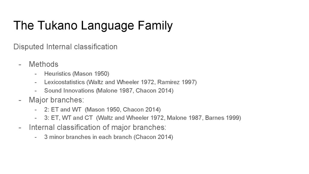
Heuristics (Mason 1950) - Lexicostatistics (Waltz and Wheeler 1972, Ramirez 1997) - Sound Innovations (Malone 1987, Chacon 2014) - Major branches: - 2: ET and WT (Mason 1950, Chacon 2014) - 3: ET, WT and CT (Waltz and Wheeler 1972, Malone 1987, Barnes 1999) - Internal classification of major branches: - 3 minor branches in each branch (Chacon 2014)
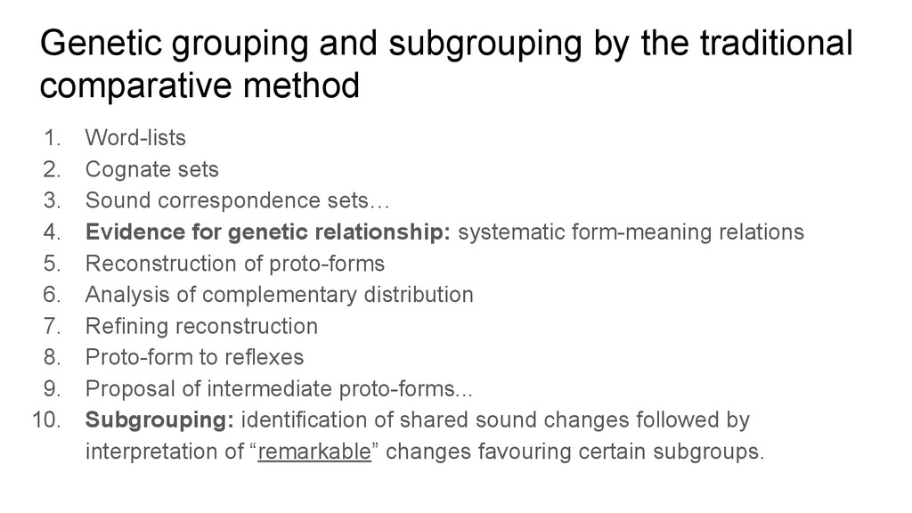
Word-lists 2. Cognate sets 3. Sound correspondence sets… 4. Evidence for genetic relationship: systematic form-meaning relations 5. Reconstruction of proto-forms 6. Analysis of complementary distribution 7. Refining reconstruction 8. Proto-form to reflexes 9. Proposal of intermediate proto-forms... 10. Subgrouping: identification of shared sound changes followed by interpretation of “remarkable” changes favouring certain subgroups.
set Kor Sek Sio Mai Tan Bas Des Kub Tuk Kar Wan P-T Gloss pia p’ia p’ia ʔbia bia bia bia bia bia bia bia *p’ia CHILI jeha jeha jiha jiha - jiba jeba jeba je’pa jepa ja’pa *jip’a LAND/ GROUND
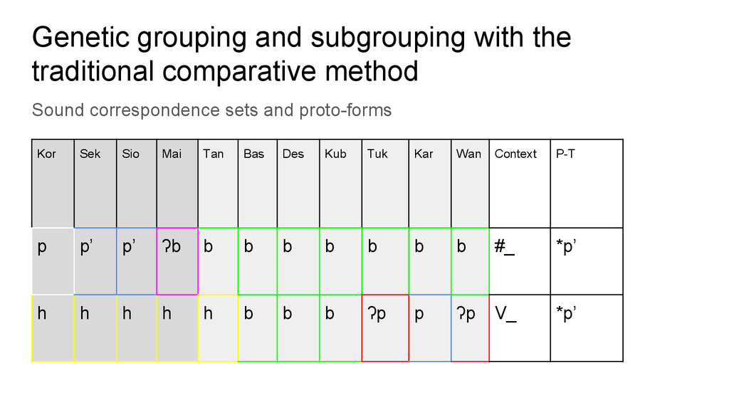
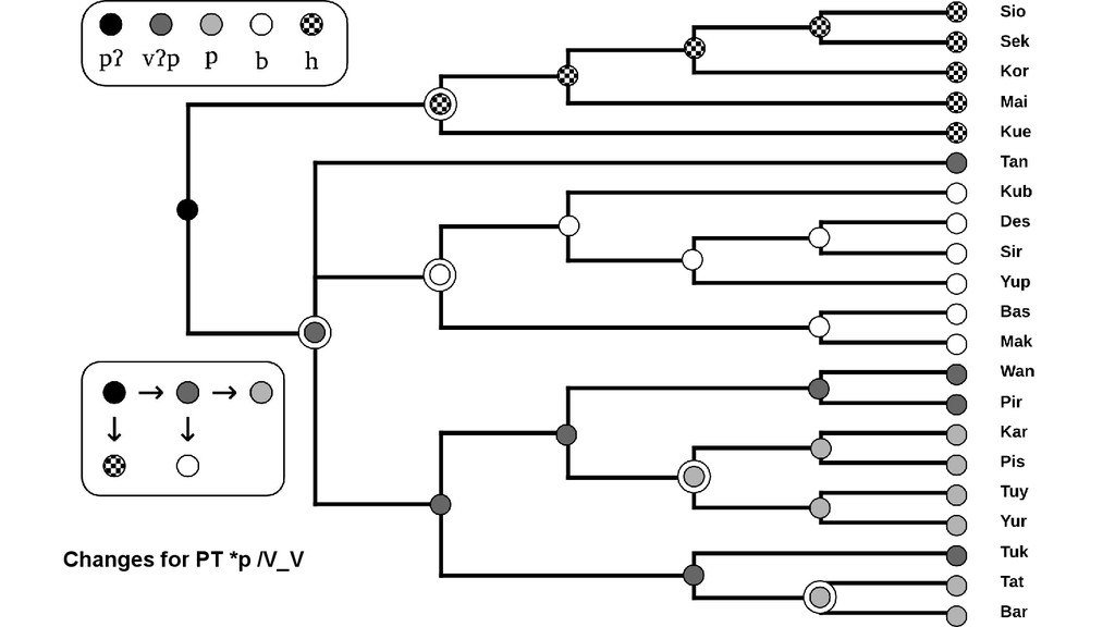
correspondence sets and proto-forms Kor Sek Sio Mai Tan Bas Des Kub Tuk Kar Wan Context P-T p p’ p’ ʔb b b b b b b b #_ *p’ h h h h h b b b ʔp p ʔp V_ *p’
Homoplasy: Not all sound changes occur only once, they can occur multiple times, and some are so frequent that they do not provide any evidence for subgrouping (think of kentum-satem languages). But there’s often disagreement among scholars as to what are innovations and what not. • What counts as “remarkable”: Scholars have not come up with a rigorous procedure that would justify why some innovations should be more important for subgrouping than others. • Circularity: Since reconstruction usually involves a certain amount of subgrouping (at least in the researcher’s heads), one runs the risk of making circular arguments for a certain subgroup due to a certain reconstruction. • Risk of cherry picking: In the end, all scholars run the danger of selecting innovations just according to their original hypotheses.
making the subgrouping enterprise more objective: - “Remarkable” is replaced by a definite principle of overall uniqueness: subgroups are established by the greatest number of more unique changes shared by a set of languages - Homoplasy is captured as the most frequent changes recurring over a set of languages that also share more unique changes - No personal bias towards cherry picking Circularity between reconstruction and subgrouping is to some degree still present, but... - “Phonetic Drifts” give a phonetic measure of the likelihood of a change - The algorithm evaluates other changes that were not at the focus of the analyst when establishing subgroupings
sets: 150 cognates iii. extracting sound correspondences: 33 sets iv. reconstruction of proto-sounds: 18 consonants and 42 reflexes v. Preparation of “phonetic drifts” for creating networks of sound transitions
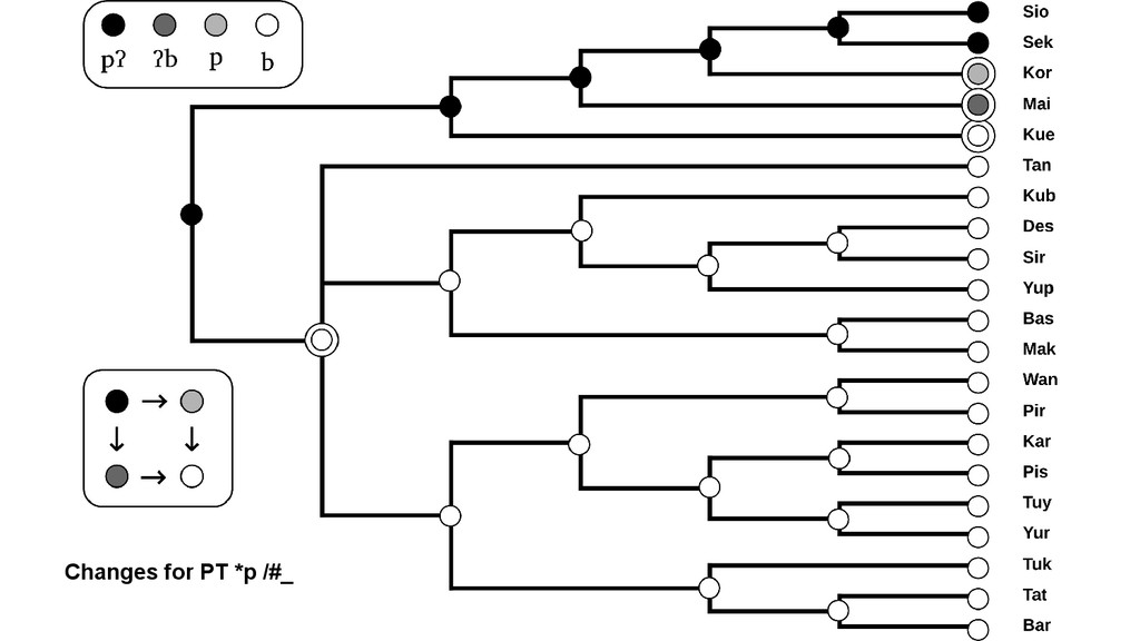
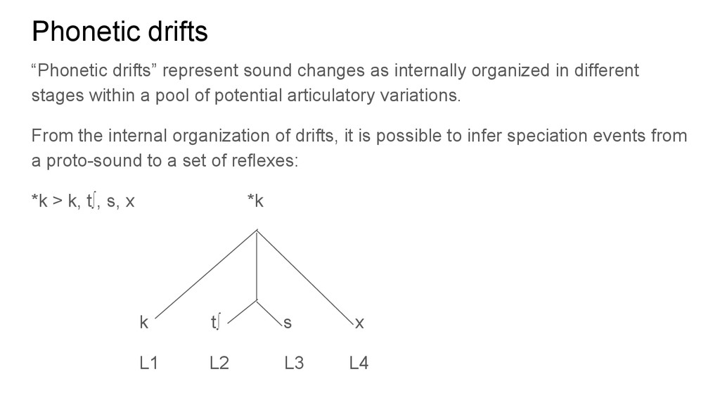
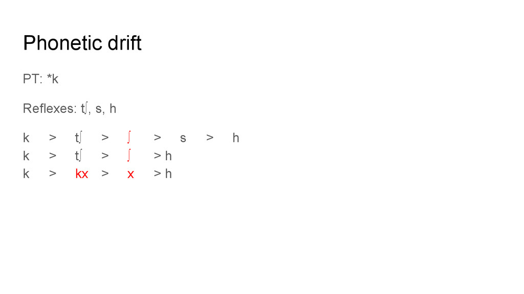
in different stages within a pool of potential articulatory variations. From the internal organization of drifts, it is possible to infer speciation events from a proto-sound to a set of reflexes: *k > k, t∫, s, x *k k t∫ s x L1 L2 L3 L4
nature of sound changes, which are Regular: or at least overwhelmingly Gradual: following more or less discrete steps from T1 to T2… Tn Phonetically blind: overwhelmingly following from universal principles of phonetics Directional: A > B but B > A
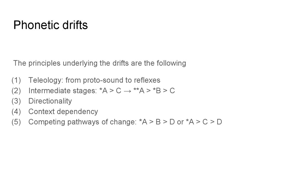
(1) Teleology: from proto-sound to reflexes (2) Intermediate stages: *A > C → **A > *B > C (3) Directionality (4) Context dependency (5) Competing pathways of change: *A > B > D or *A > C > D
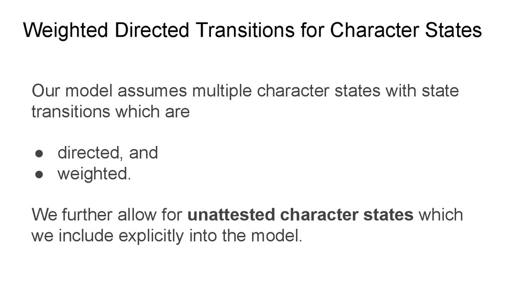
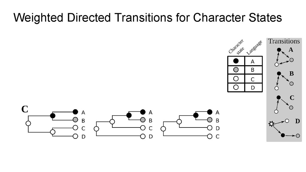
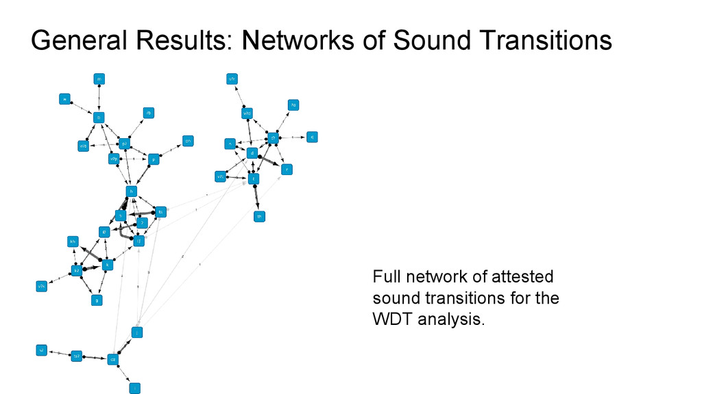
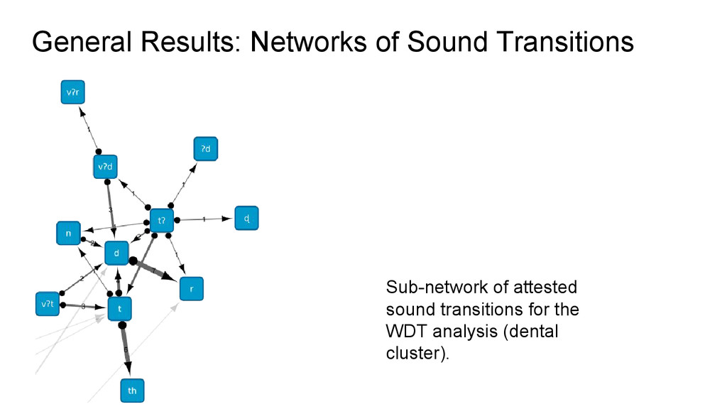
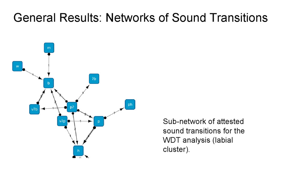
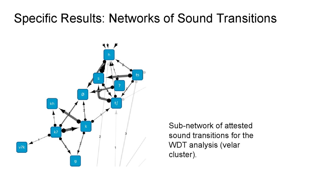
character states with state transitions which are • directed, and • weighted. We further allow for unattested character states which we include explicitly into the model.
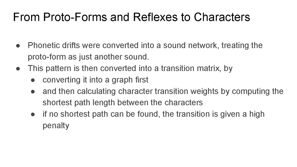
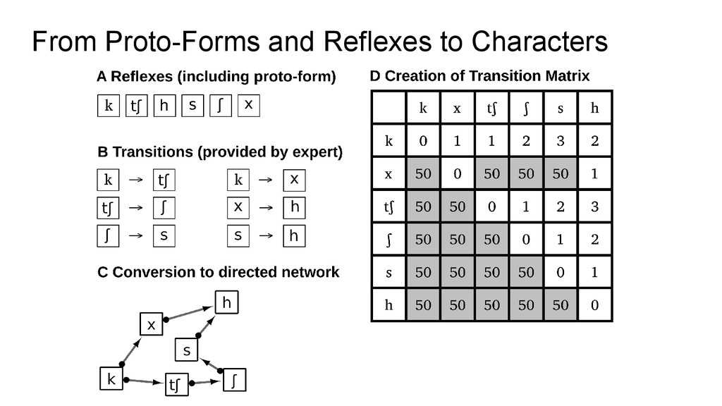
converted into a sound network, treating the proto-form as just another sound. • This pattern is then converted into a transition matrix, by • converting it into a graph first • and then calculating character transition weights by computing the shortest path length between the characters • if no shortest path can be found, the transition is given a high penalty
through the whole tree space when dealing with more than 10 languages, we need to search heuristically. The strategy we use follows the following schema: • start from a random tree, and ◦ create more trees by swapping nodes in the tree ◦ retain the best trees (in terms of parsimony scores) and create more trees from them ◦ create more random trees to avoid to get stuck in a local maximum • stop the tree search and return the best trees, if the researcher has had enough
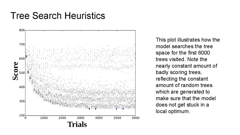
for the first 6000 trees visited. Note the nearly constant amount of badly scoring trees, reflecting the constant amount of random trees which are generated to make sure that the model does not get stuck in a local optimum. Tree Search Heuristics
as a LingPy plugin (later to be included regularly in LingPy). • We analyzed three different models (searching 500 000 trees for each), in order to check for the effects of directionality and weights in networks: ◦ FITCH: a simple parsimony that penalizes every transition with 1 ◦ SANKOFF: a weighted parsimony model that penalizes transitions by calculating the shortest path in the sound transition network, but with the sound transition network being treated as an undirected network ◦ WDT (weighted directed transitions): The model which we described before. • We evaluate the performance of each model by comparing the reconstruction quality (ancestral state reconstruction for the best trees), and the trees themselves (qualitative evaluation).
a given analysis (a tree or a set of trees), we can calculate for each sound transition how frequently it occurs in the data for the given tree. This is interesting both with respect to questions regarding sound change frequencies, but also with respect to the quality of our analysis, since we would assume that those changes which occur most frequently are also those changes which are generally frequent and lead to high degrees of homoplasy in parsimony analyses.
created to allow for a quick inspection of the results. • It shows individual evolutionary scenarios inferred for each of the models and the corresponding consensus tree. • It shows also a summary of each model with all changes inferred for each node and a detailed listing of those sounds that have changed by then according to the given model. • The application can be launched via: http://digling.org/tukano/
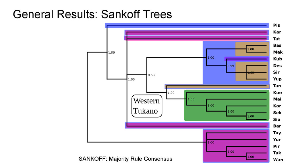
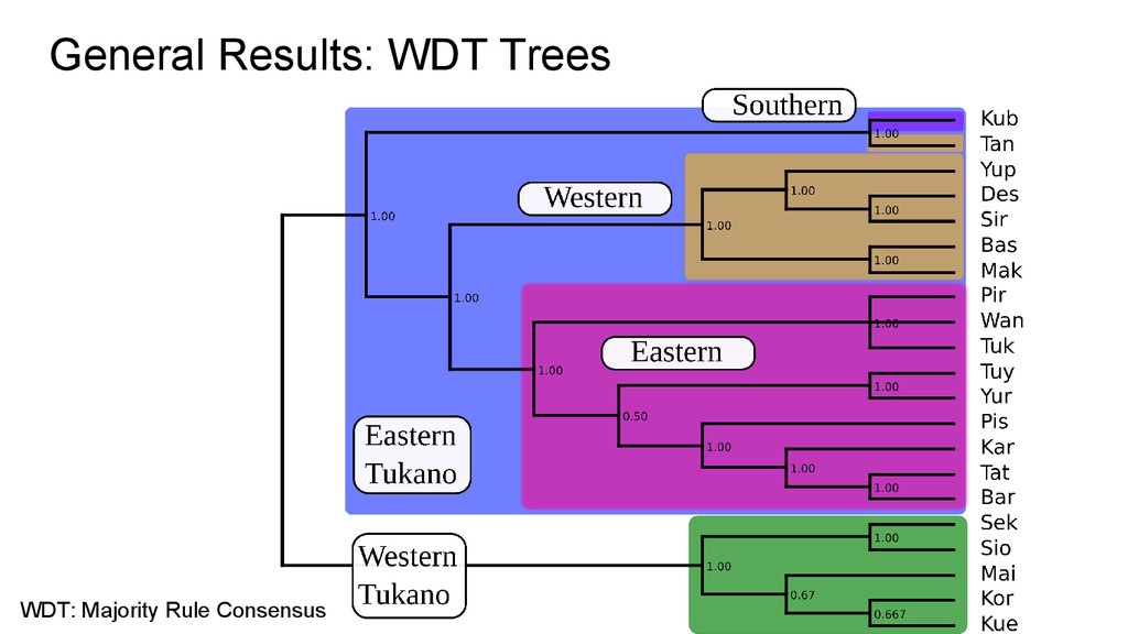
intermediate subgroups - Only surface similarities seem to have influenced the tree - A little better performance regarding more shallow subgroups - Perfect match with manual classification regarding Western-ET subgroup
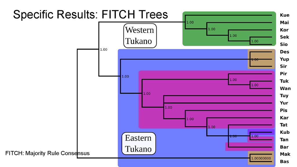
classification - ET and WT was not fully captured - ET languages BAS and MAK were wrongly classified as an outgroup - Good tree for WT and E-ET languages
split was neatly captured! - WT internal classification matches perfectly with manual classification - 3 ET subgroups! - Kub and Tan as an ET outgroup, confirming alternative expectations! - Very consistent subgrouping in Western-ET and Eastern-ET
each character (“local” vs. “global” networks) ◦ constraining vs. expanding intermediate stages in phonetic transitions ◦ weighting sound transitions, e.g.: ▪ assimilation +1 incrementation vs. dissimilation +5 incrementation ▪ articulatorily biased change +1 vs. acoustically biased change +2 ◦ other linguistic families: ▪ widely known, e.g. Romance vs. poorly known, e.g. Arawak ▪ shallow vs. deeper time depth ▪ few (around 10) vs. many languages (40+) Research and database on the typology of sound changes Directionality seems to be the key. Do we get directionality into probabilistic models?