Automatic Cognate Detection: Evaluation, Benchmarks, and Probabilities

Talk by Luke Maurits, Simon Greenhill, and Johann-Mattis List, presented at the workshop "Towards a Global Language Phylogeny", 21-23 October, Max Planck Institute for the Science of Human History, Jena.

Transcript

1. Automatic Cognate Detection Evaluation, Benchmarks, and Probabilities Luke Maurits, Johann-Mattis List, and Simon Greenhill
2. Outline 1. Evaluation a. Overview on LingPy’s cognate detection methods b. Introducing a new method based on Infomap community clustering c. Testing the method on a newly compiled testset 2. Benchmarks a. Pointing to the importance of having good benchmark databases b. Show an example of how a Cognate Detection Benchmark Database could look like c. Introducing the idea of having a series of benchmark databases in GlottoBank 3. Probabilities a. Towards a Bayesian approach b. The Chinese Restaurant Process c. MAP approach and beyond
3. Evaluation
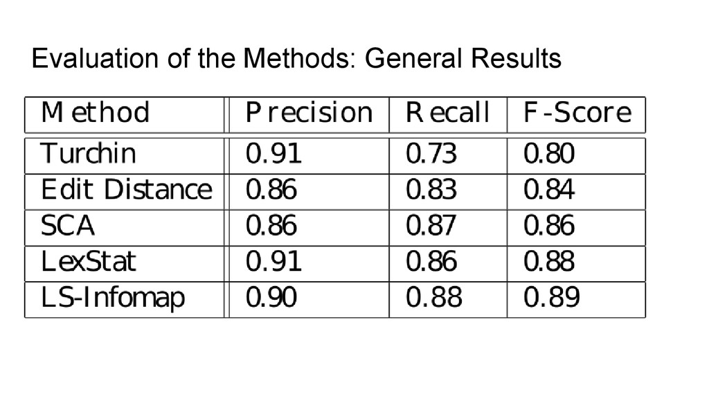
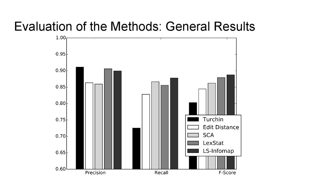
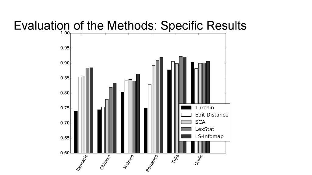
4. LingPy’s Cognate Detection Methods • LingPy currently offers four cognate detection methods ◦ Turchin et al. (2010): simple sound class method, first two sounds decide about cognacy ◦ Edit Distance: Normalized edit distance is calculated for all word pairs and the results are partitioned into cognate sets (using flat UPGMA clustering) ◦ SCA: SCA distances (List 2012) are calculated for all word pairs and the results are partitioned into cognate sets (using flat UPGMA) ◦ LexStat: Language specific scoring schemes (close to sound correspondences, effectively log-odds) are calculated and partitioned into cognate sets (UPGMA) • The methods show an increasing accuracy, but also an increasing computational cost
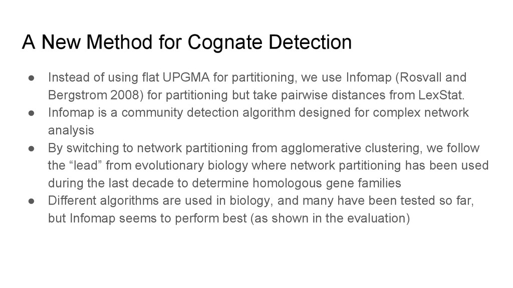
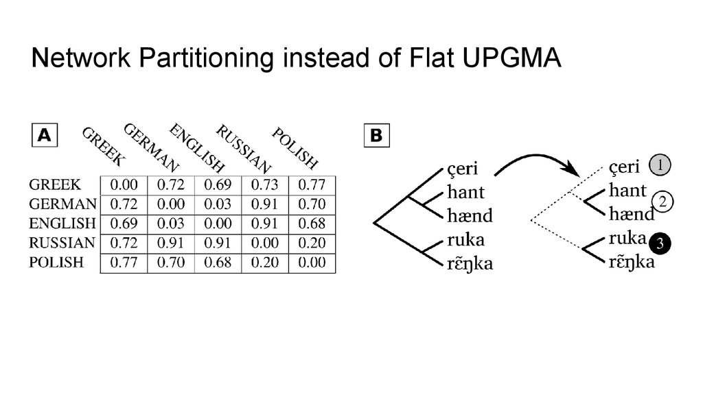
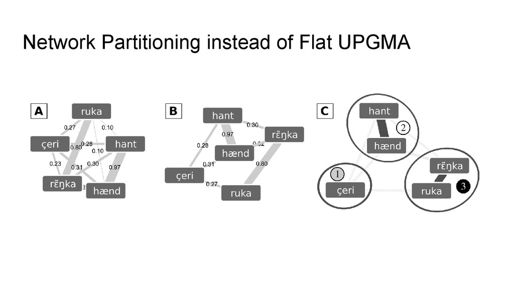
5. A New Method for Cognate Detection • Instead of using flat UPGMA for partitioning, we use Infomap (Rosvall and Bergstrom 2008) for partitioning but take pairwise distances from LexStat. • Infomap is a community detection algorithm designed for complex network analysis • By switching to network partitioning from agglomerative clustering, we follow the “lead” from evolutionary biology where network partitioning has been used during the last decade to determine homologous gene families • Different algorithms are used in biology, and many have been tested so far, but Infomap seems to perform best (as shown in the evaluation)
6. Network Partitioning instead of Flat UPGMA
7. Network Partitioning instead of Flat UPGMA
8. Evaluating the Performance on a New Testset
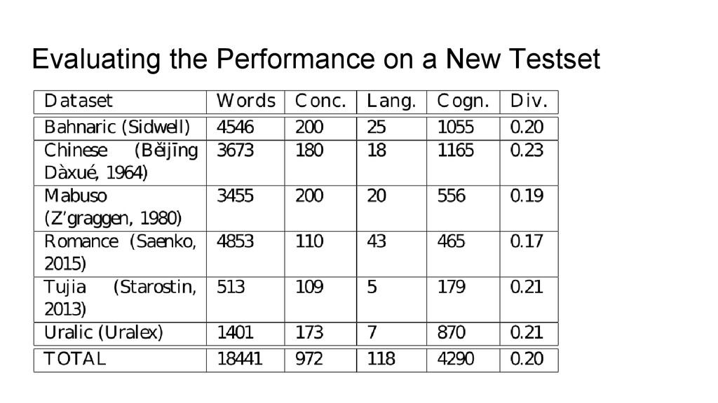
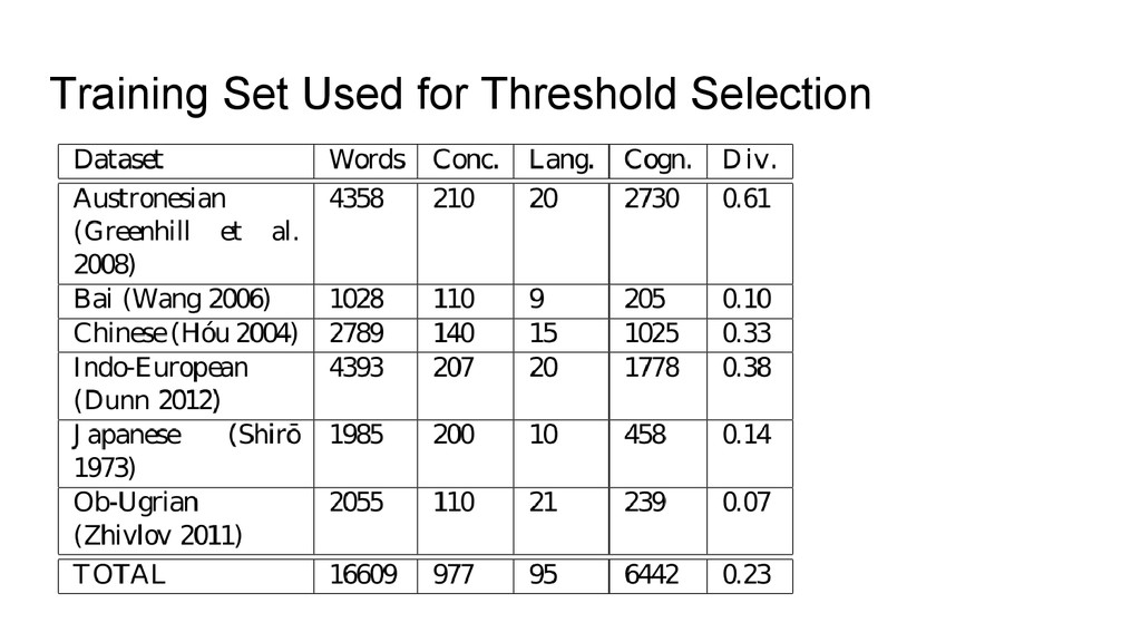
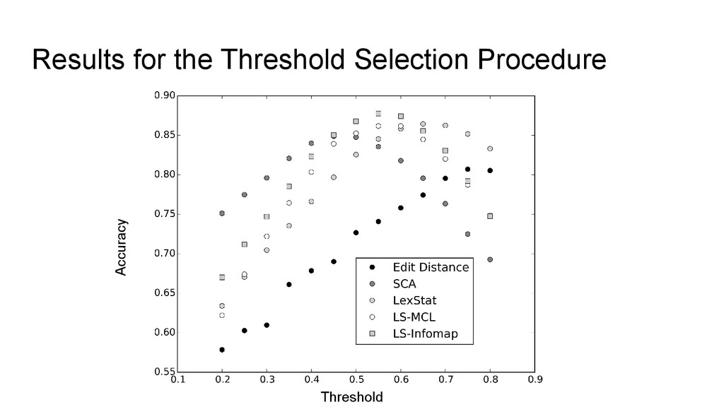
9. Problem of Threshold Selection • Apart from the Method by Turchin et al. (2010), all three remaining and the new method require that we know where to set the threshold. • In order to test how well the methods perform, we need to find a way to determine some threshold in some “objective” way • Luke will talk about this in greater detail • For our testing of the new dataset and the new methods, we decided to use a training set (List 2014) to determine the “best” threshold for each of the methods. • While testing the three LingPy methods which require a threshold, we also tested the new method (LS-Infomap) and an alternative method (LS-MCL, based on Markov Clustering, Dongen 2000).
10. Training Set Used for Threshold Selection
11. Results for the Threshold Selection Procedure Accuracy Threshold
12. Evaluation of the Methods: General Results
13. Evaluation of the Methods: General Results
14. Evaluation of the Methods: Specific Results
15. Intermediate Conclusion • The results seem to be already good enough to be used for computer- assisted language comparison (do a pre-processing with cognate detection analyses and later having them refined by experts) • The results show that we might be able to push the barrier: switching to better partitioning algorithms increased the results by 1 point. What happens if we also manage to refine the calculation of the similarity scores?
16. Benchmarks
17. Towards a Cognate Detection Benchmark Database • Benchmark databases are essential to train, test, and evaluate our algorithms • So far, there are not many benchmark databases which could be used for our tasks • With the new data we prepared for this study, and the data that was compiled to test LingPy (List 2014), there are already 18 different datasets which are ◦ in more or less clean phonetic encoding ◦ are segmentized ◦ are tagged for cognacy • We think these should be published as a benchmark database for cognate detection (BDCD, or “LexiBench”?) • In this way, we maintain comparability with other algorithms that might be proposed, and we ease the creation of alternative approaches
18. Benchmark Database for Cognate Detection: Demo • This is a first demo version, on how a benchmark database could look: • http://digling.org/lexibench/ • It is nothing special, and we do not need anything really special, but we should get the data out there, so that people know they can use it...
19. Benchmark Databases in General • There is a Benchmark Database for Phonetic Alignment (List and Prokić 2014), which will be extended in 2015 (scholars start providing data). • There could be more benchmark databases for other tasks that are relevant for us. • We may think of establishing a general “brand” for benchmark databases, summarized under, say “GlottoBench” (and the alignment benchmark can be directly included there). • Alternatively, we can go for separate benchmarks. • But what we need is to spread the word that there is data that people can use for developing and testing their algorithms. • Otherwise, computational linguists will keep on using the Dyen database in an uppercase version to check how well their algorithms detect cognates...
20. Probabilities
21. Toward a Bayesian approach • Deterministic methods like those just outlined have some drawbacks (and also advantages!) • We only get black-and-white results from them. • Two words are either definitely cognate, or they are definitely not. • By adjusting thresholds we can trade off between Type I and Type II errors. • But we must apply a single threshold to the entire dataset. • The thresholds are essentially arbitrary, and choosing one for a new dataset is difficult.
22. Virtues of probabilistic modelling • Probabilistic models can overcome many of these shortcomings (usually at the greater computational expense). • We can get more nuanced results like “these two words are cognate with probability 0.72” • We can also have the model attempt to “learn its own thresholds” from the data, removing the need to guess arbitrary thresholds for new datasets.
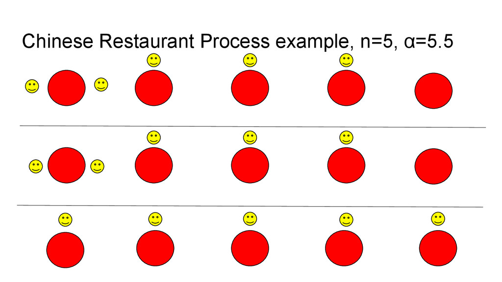
23. Introducing the Chinese Restaurant Process • The CRP is whimsically-named discrete-time stochastic process. • Imagine a Chinese restaurant with an infinite number of tables. • Imagine each table has an infinite number of seats. • Customers enter the restaurant and are seated one at a time. • Where each customer sits is randomly determined.
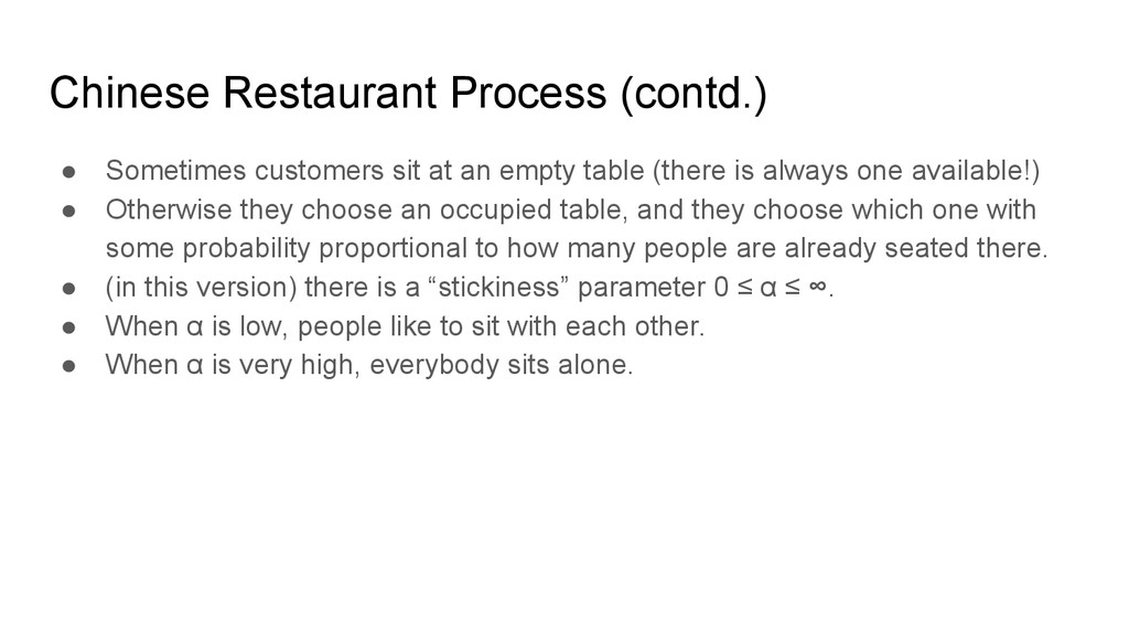
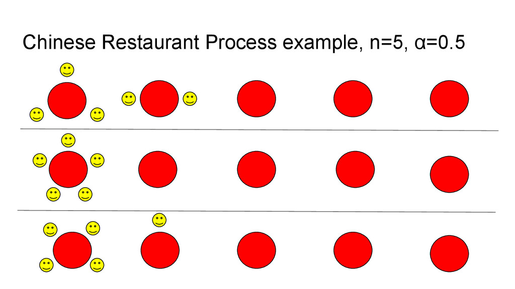
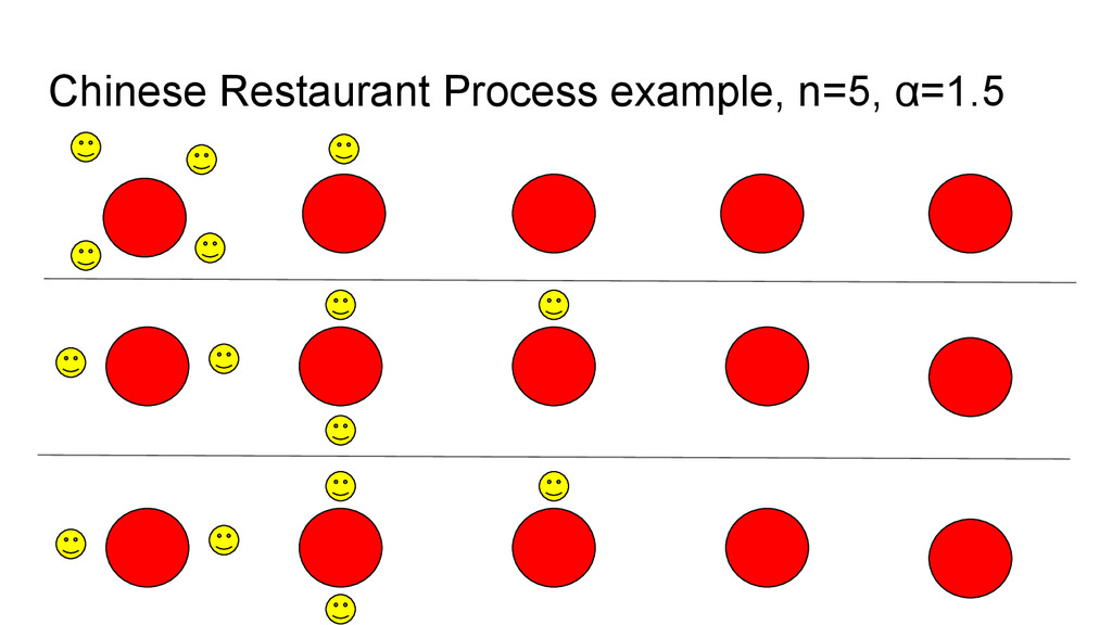
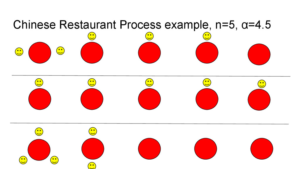
24. Chinese Restaurant Process (contd.) • Sometimes customers sit at an empty table (there is always one available!) • Otherwise they choose an occupied table, and they choose which one with some probability proportional to how many people are already seated there. • (in this version) there is a “stickiness” parameter 0 ≤ α ≤ ∞. • When α is low, people like to sit with each other. • When α is very high, everybody sits alone.
25. Chinese Restaurant Process example, n=5, α=0.5
26. Chinese Restaurant Process example, n=5, α=1.5
27. Chinese Restaurant Process example, n=5, α=2.5
28. Chinese Restaurant Process example, n=5, α=4.5
29. Chinese Restaurant Process example, n=5, α=5.5
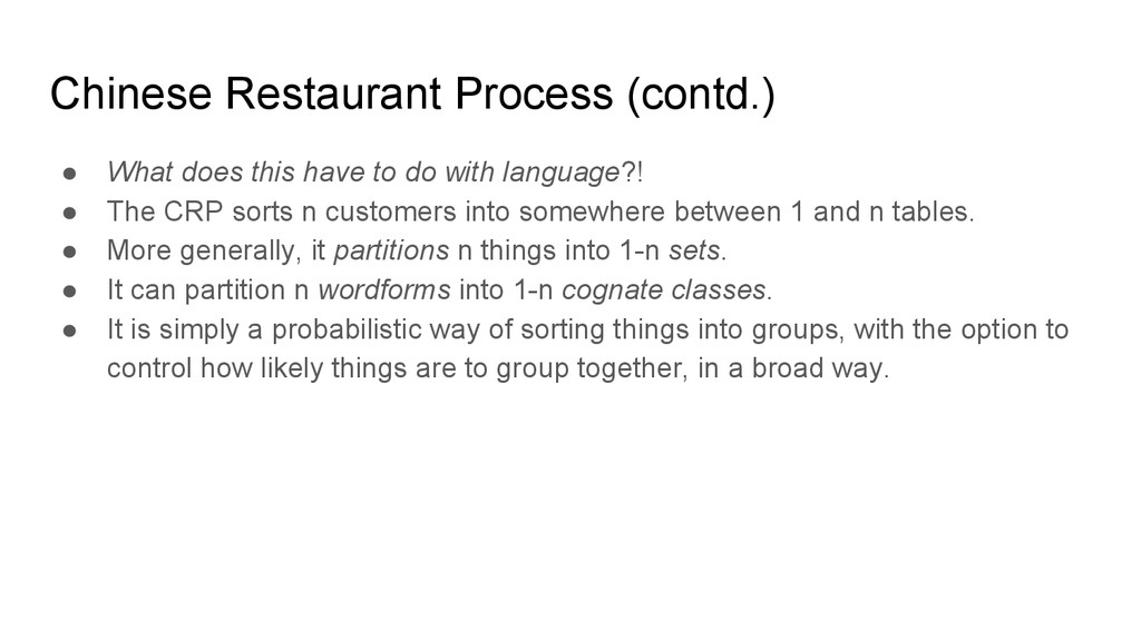
30. Chinese Restaurant Process (contd.) • What does this have to do with language?! • The CRP sorts n customers into somewhere between 1 and n tables. • More generally, it partitions n things into 1-n sets. • It can partition n wordforms into 1-n cognate classes. • It is simply a probabilistic way of sorting things into groups, with the option to control how likely things are to group together, in a broad way.
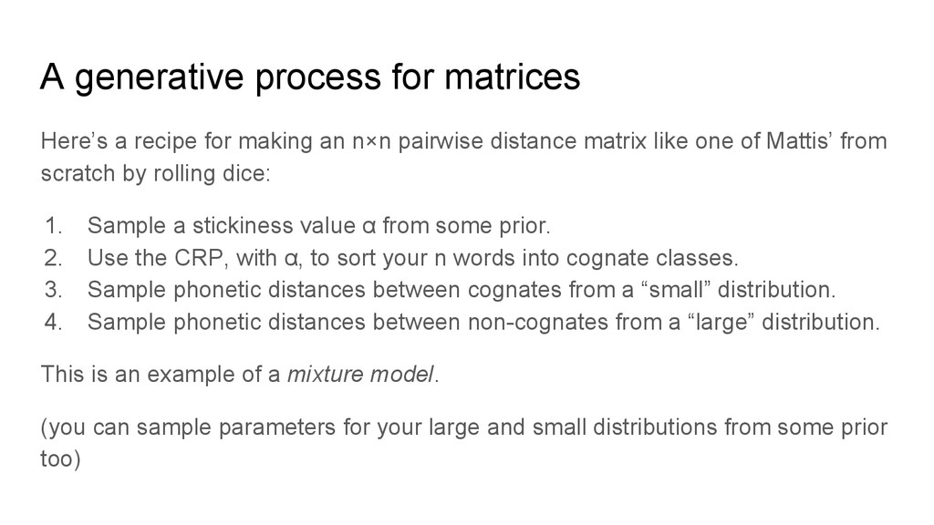
31. A generative process for matrices Here’s a recipe for making an n×n pairwise distance matrix like one of Mattis’ from scratch by rolling dice: 1. Sample a stickiness value α from some prior. 2. Use the CRP, with α, to sort your n words into cognate classes. 3. Sample phonetic distances between cognates from a “small” distribution. 4. Sample phonetic distances between non-cognates from a “large” distribution. This is an example of a mixture model. (you can sample parameters for your large and small distributions from some prior too)
32. Bayes flip! • We just outlined a way to stochastically generate phonetic distance matrices. • We we already have (or can get) phonetic distance matrices. • Those are our data! • The value of generative models is that we can use Bayes’ theorem to reverse them. P(H|D) ∝ P(D|H) • Here H is our cognate classification (and α, and any distribution parameters)
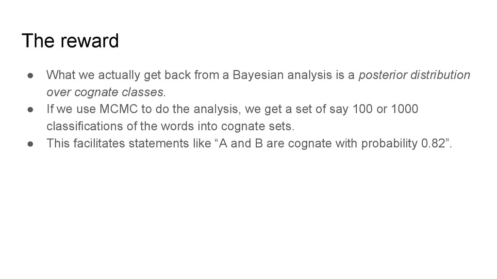
33. The reward • What we actually get back from a Bayesian analysis is a posterior distribution over cognate classes. • If we use MCMC to do the analysis, we get a set of say 100 or 1000 classifications of the words into cognate sets. • This facilitates statements like “A and B are cognate with probability 0.82”.
34. Does it work? • We get back uncertain estimates of cognate classes. • So we can’t immediately compute precision, recall or F scores against gold standards. • For the sake of easy and direct comparison to gold standards or existing methods, we need a way to distil our uncertain estimates into clear “consensus classes” (cf. consensus trees). • How best to do this is an interesting research problem in itself
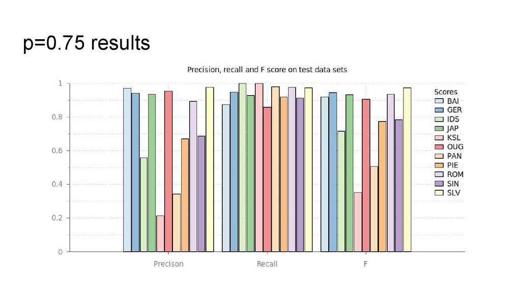
35. A simple first effort • The MAP results feature good precision but mediocre recall. • We need to introduce a little more “slack”. • Here’s an off-the-cuff approach: • For each wordform, build a cognate set out of all those forms which are cognate with p ≥ 0.75, say. • Look for wordforms assigned to multiple cognate classes (bad). • Keep the form in the class with the highest product of pairwise probabilities
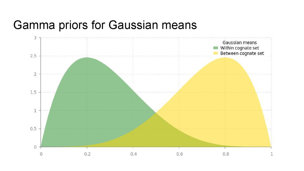
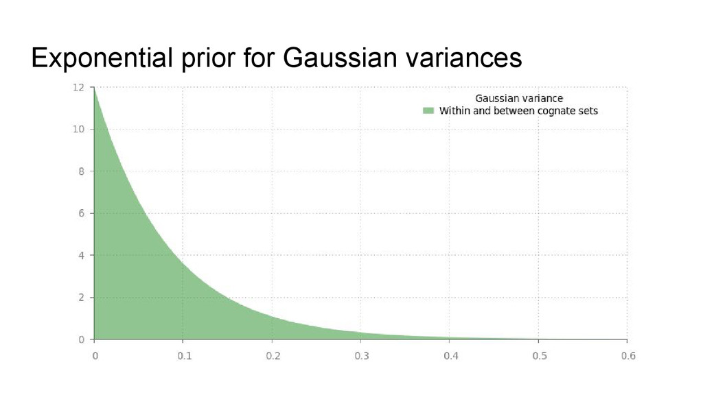
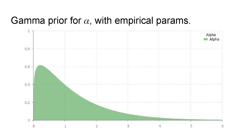
36. A few more details • We test a particular form of the generative model • Our “big” and “small” distributions are Gaussians, with separate means and variances. • The two distributions have different priors on their means (favouring large or small values), and the same priors on their variances (favouring lower values) • The prior over α is based on some gold standard classifications.
37. Gamma priors for Gaussian means
38. Exponential prior for Gaussian variances
39. Gamma prior for , with empirical params.
40. p=0.75 results
41. Thresholds strike back • Of course, the threshold can be varied from 0.75. • As threshold is lowered, we trade precision for recall. • But wait, weren’t we trying to get rid of arbitrary thresholds?! • This is not so bad: the threshold has a principled interpretation which holds across data sets (cf the arbitrary use of 0.05 significance in hypothesis testing).
42. Future work • One shortcoming of this method is the independence of the restaurants • All restaurants share the same α, so are equally “clumpy” or “spread out” • But there is no requirement for clumpings to be consistent across restaurants, as we may expect. • We don’t just want people to always sit at 2 or 3 crowded tables, we want roughly the same crowds each time • A modification to the CRP may help with this?
43. More future work • An unexplored question: how can we infer trees using this system? • We can compute consensus cognate classes as an intermediate step and then use Covarion or Dollo models in the traditional way. • But this throws away the uncertainty information we have worked so hard to get! • Can we do away with the intermediate step entirely and develop a tree-based generative model for distance matrices?
44. Thank you! • Any questions?