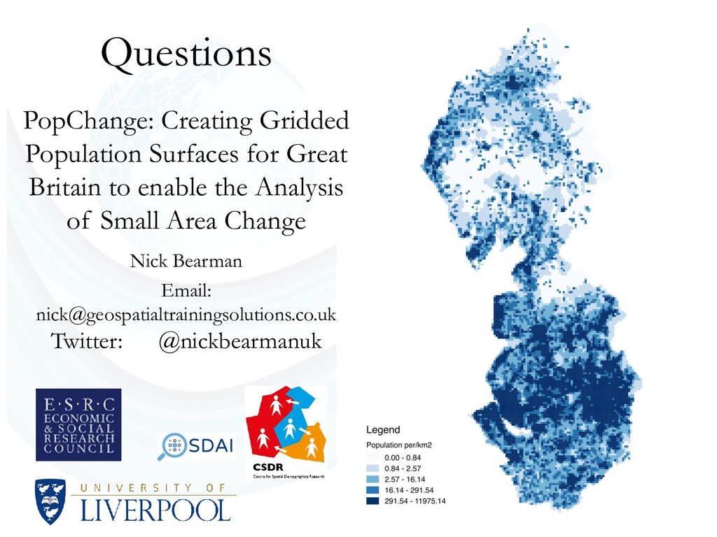
the Analysis of Small Area Change Nick Bearman Project team: Chris Lloyd*, Gemma Catney* and Paul Williamson, University of Liverpool, UK *Now Queens University, Belfast Email: [email protected] ¦ Twitter: @nickbearmanuk
started 2014-2015 • I worked on this 2015-2016 • Lots of potential to be developed • But…. I moved / Chris Lloyd moved….. • Now working: • 2d/wk at CDRC, UCL Geography • 3d/wk Geospatial Training Solutions, Training & Consultancy
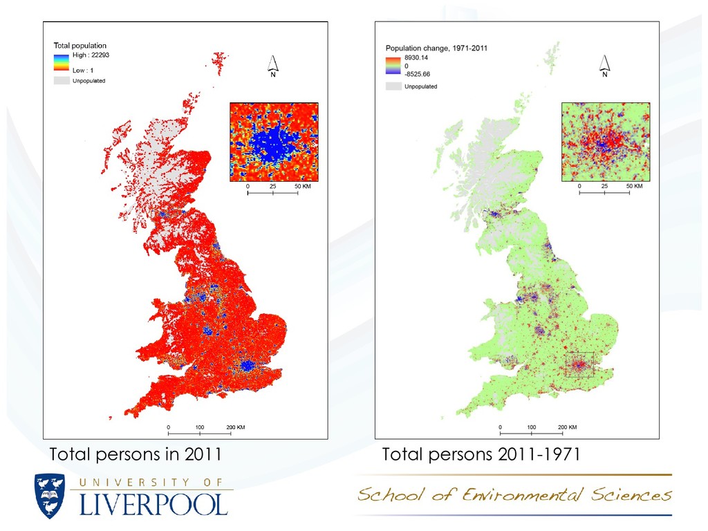
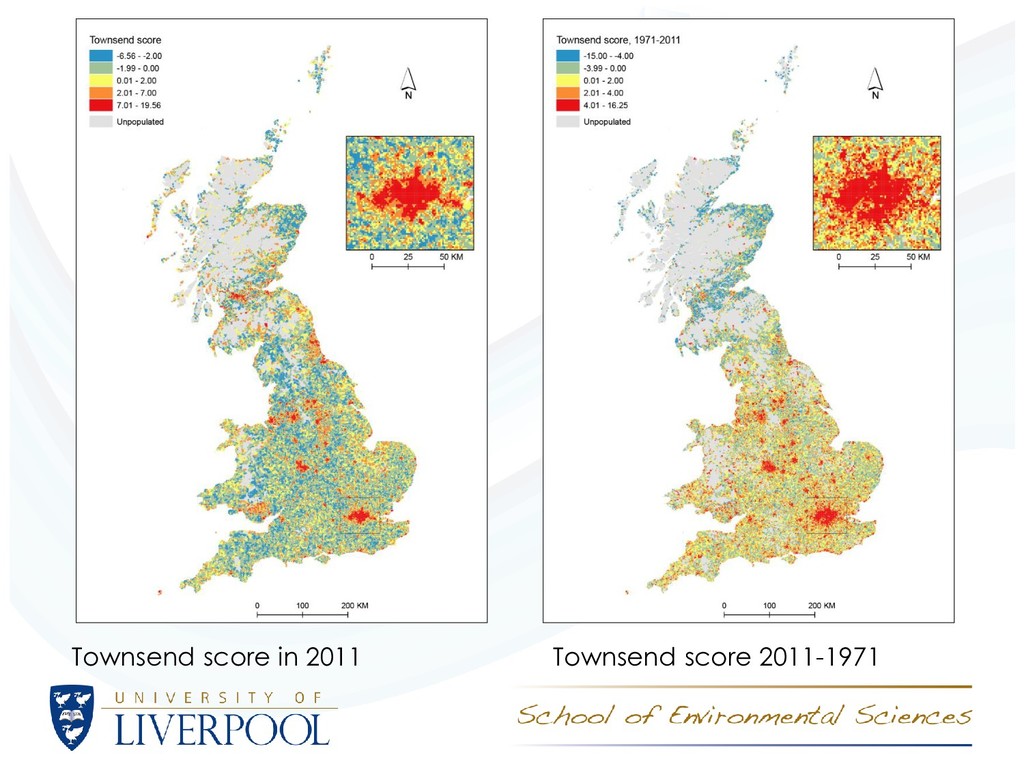
UK Censuses of 1971, 1981, 1991, 2001 and 2011 • Creation of population surfaces for Britain for all comparable variables (1km cells nationally; in Northern Ireland grid square counts for 1971-2011 are already available) • Provision of population surfaces, code in R programming language to manipulate data and an online atlas of population change
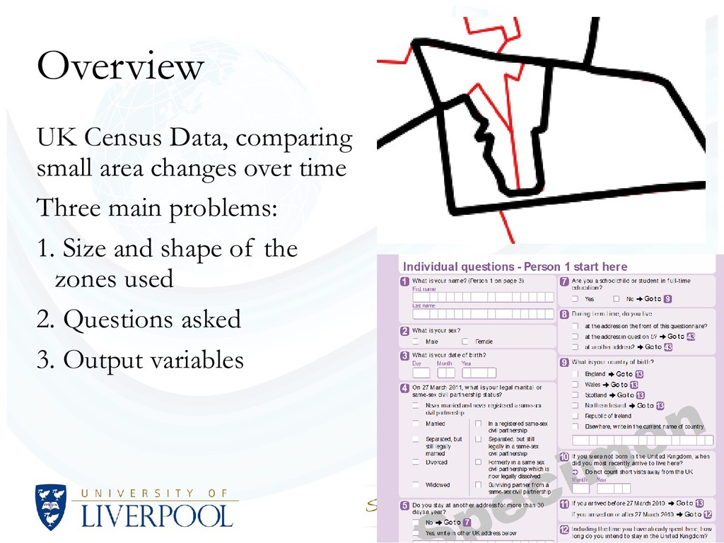
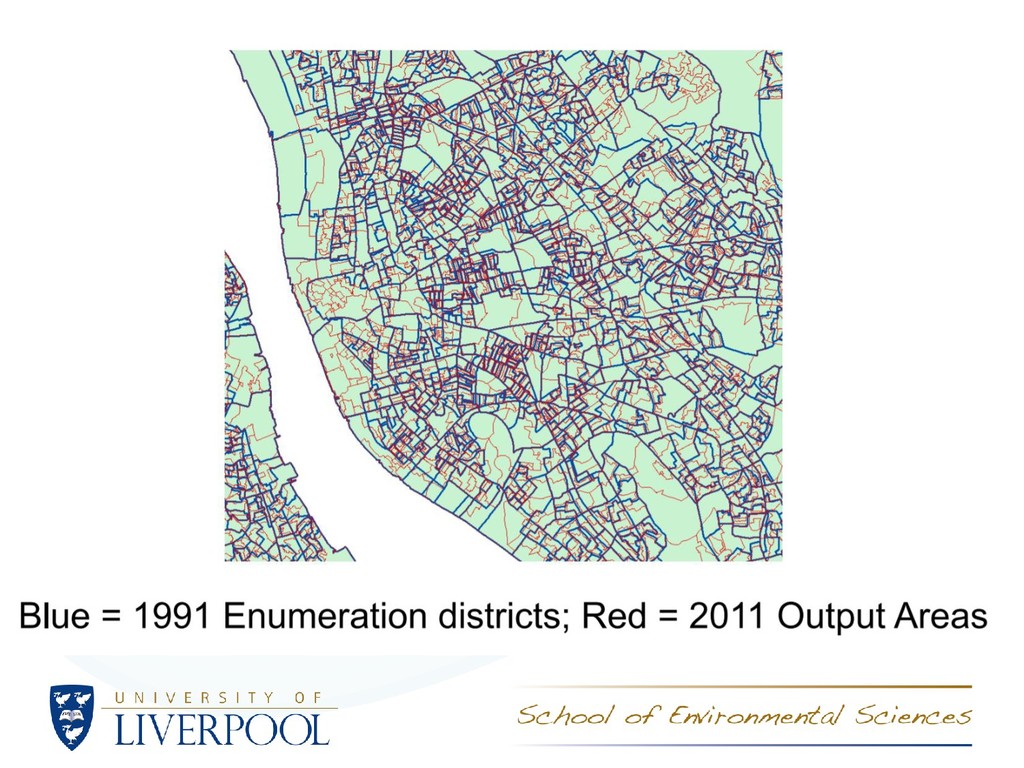
time • Splits • Merges • E.g. 2001 vs 2011 • 2.6% change* (4,561 OAs) • Black: OA 2001 • Red: OA 2011 http://www.ons.gov.uk/ons/guide-method/geography/beginner-s-guide/census/output-area--oas-/index.html
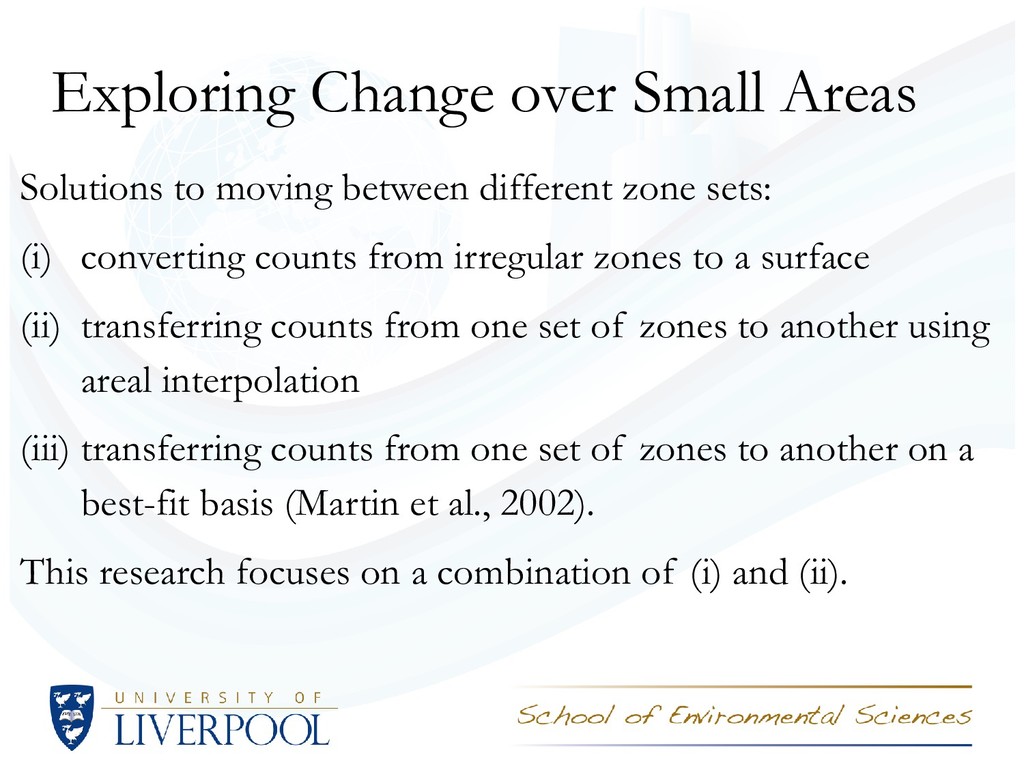
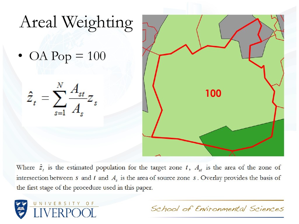
zone sets: (i) converting counts from irregular zones to a surface (ii) transferring counts from one set of zones to another using areal interpolation (iii) transferring counts from one set of zones to another on a best-fit basis (Martin et al., 2002). This research focuses on a combination of (i) and (ii).
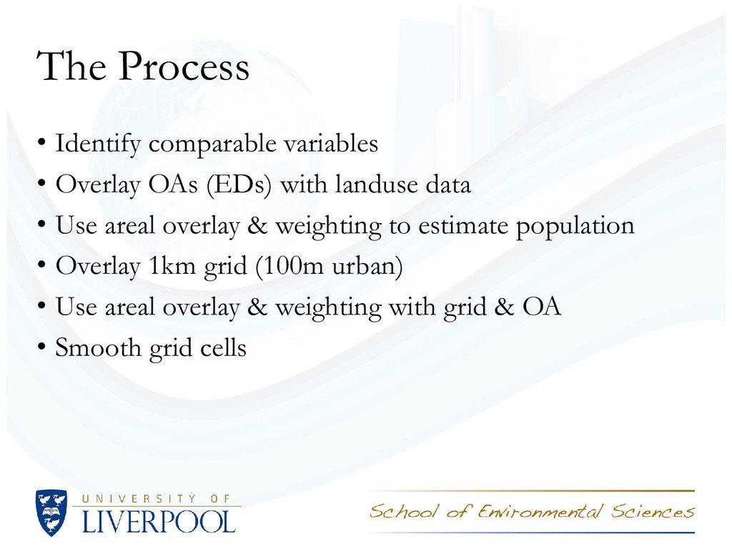
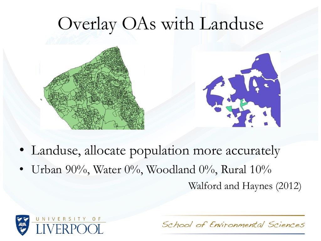
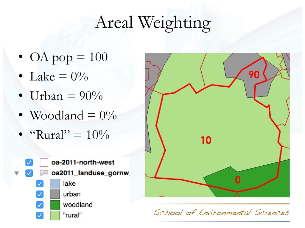
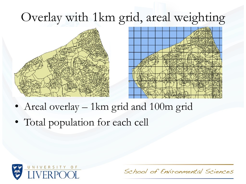
with landuse data • Use areal overlay & weighting to estimate population • Overlay 1km grid (100m urban) • Use areal overlay & weighting with grid & OA • Smooth grid cells
of the same size and shape and this makes it easier to assess scale effects without the need to account for zones whose size and shape differs • With grid cells, there are holes where there are no people; this is conceptually more sensible than zones (e.g., output areas or wards) which cover the land area completely
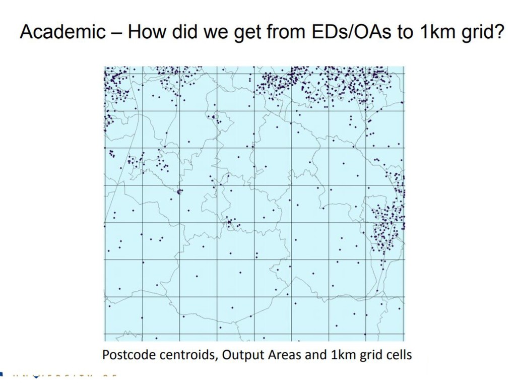
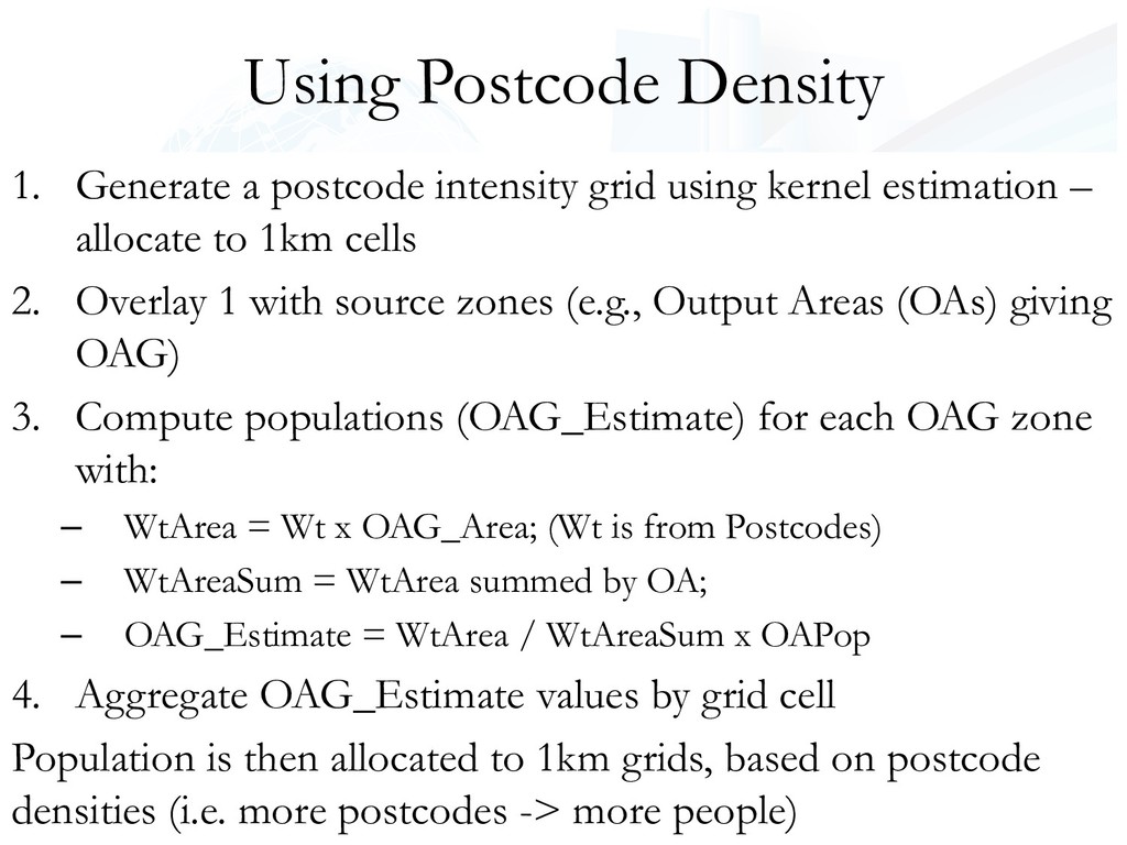
kernel estimation – allocate to 1km cells 2. Overlay 1 with source zones (e.g., Output Areas (OAs) giving OAG) 3. Compute populations (OAG_Estimate) for each OAG zone with: – WtArea = Wt x OAG_Area; (Wt is from Postcodes) – WtAreaSum = WtArea summed by OA; – OAG_Estimate = WtArea / WtAreaSum x OAPop 4. Aggregate OAG_Estimate values by grid cell Population is then allocated to 1km grids, based on postcode densities (i.e. more postcodes -> more people)
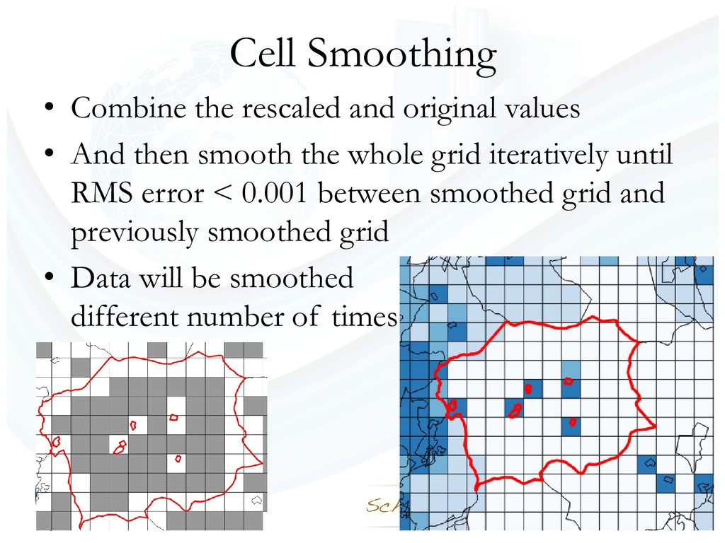
And then smooth the whole grid iteratively until RMS error < 0.001 between smoothed grid and previously smoothed grid • Data will be smoothed different number of times
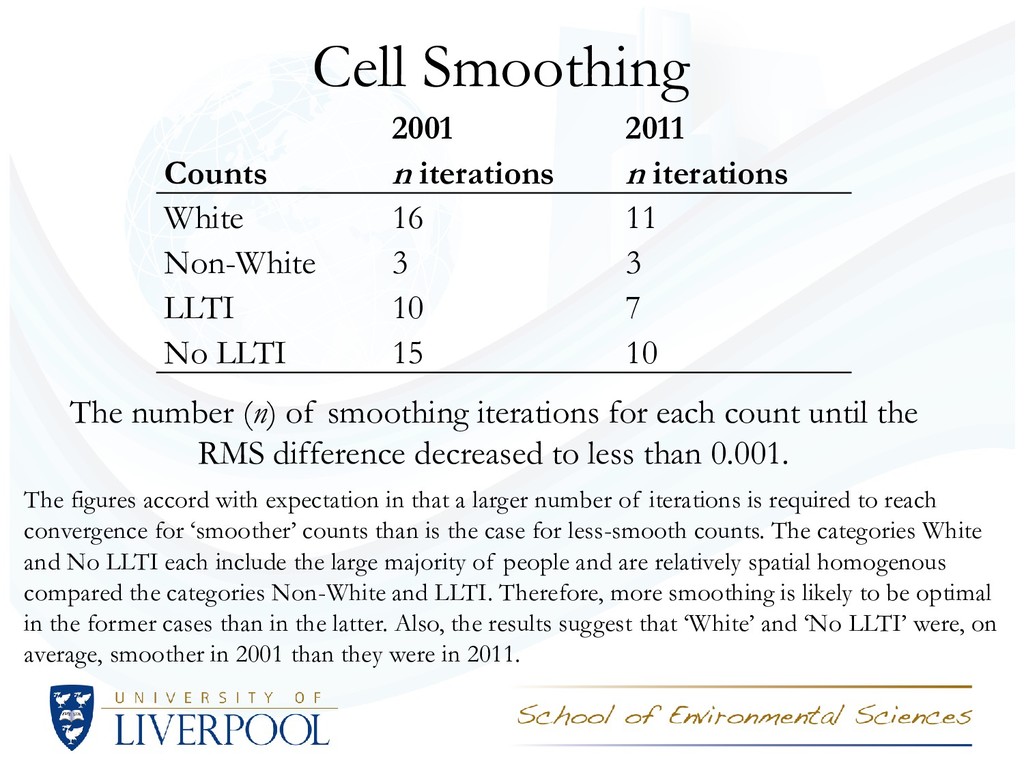
count until the RMS difference decreased to less than 0.001. 2001 2011 Counts n iterations n iterations White 16 11 Non-White 3 3 LLTI 10 7 No LLTI 15 10 The figures accord with expectation in that a larger number of iterations is required to reach convergence for ‘smoother’ counts than is the case for less-smooth counts. The categories White and No LLTI each include the large majority of people and are relatively spatial homogenous compared the categories Non-White and LLTI. Therefore, more smoothing is likely to be optimal in the former cases than in the latter. Also, the results suggest that ‘White’ and ‘No LLTI’ were, on average, smoother in 2001 than they were in 2011.
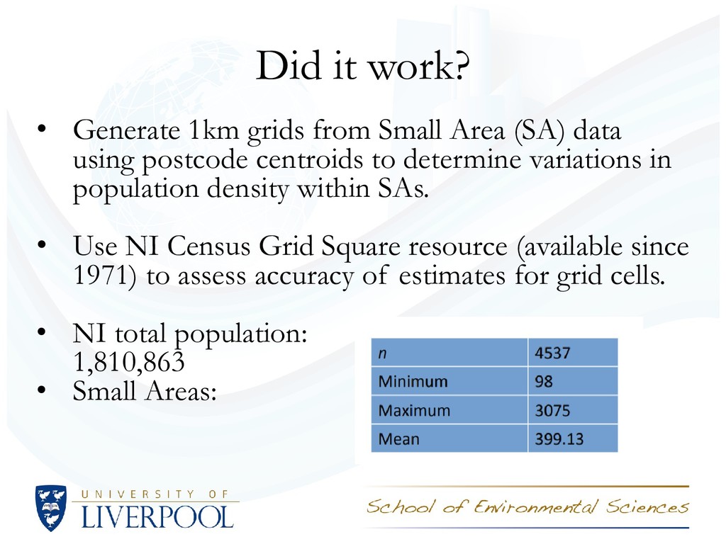
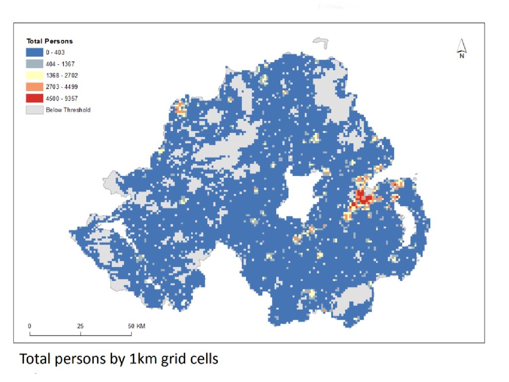
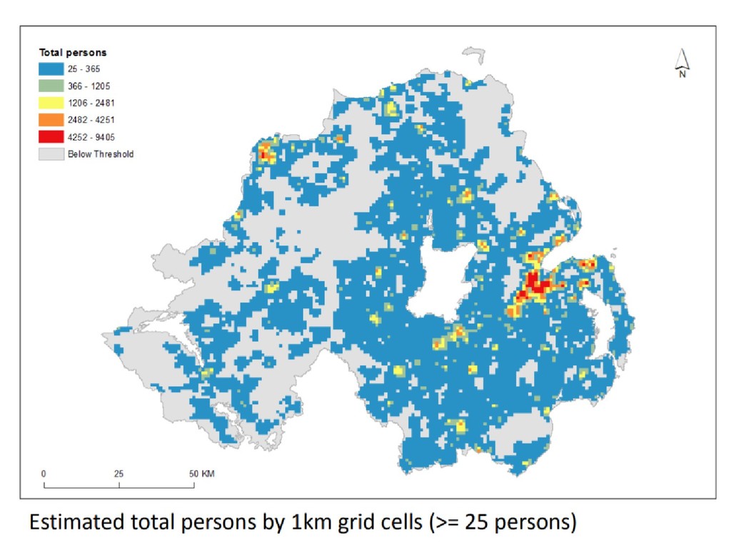
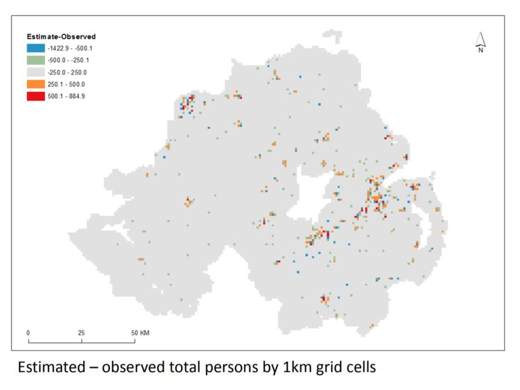
(SA) data using postcode centroids to determine variations in population density within SAs. • Use NI Census Grid Square resource (available since 1971) to assess accuracy of estimates for grid cells. • NI total population: 1,810,863 • Small Areas:
more non-Census (e.g. admin data) • Papers being finalised on changes in: – (1) deprivation, (2) country of birth and ethnicity, and (3) self-reported health (Emily Dearden's PhD) • Briefing on housing spaces (overcrowding) • Outputs in LSOA/DZ, more relevant to policy. • Onoing work in SA, spatial inequalities, grids
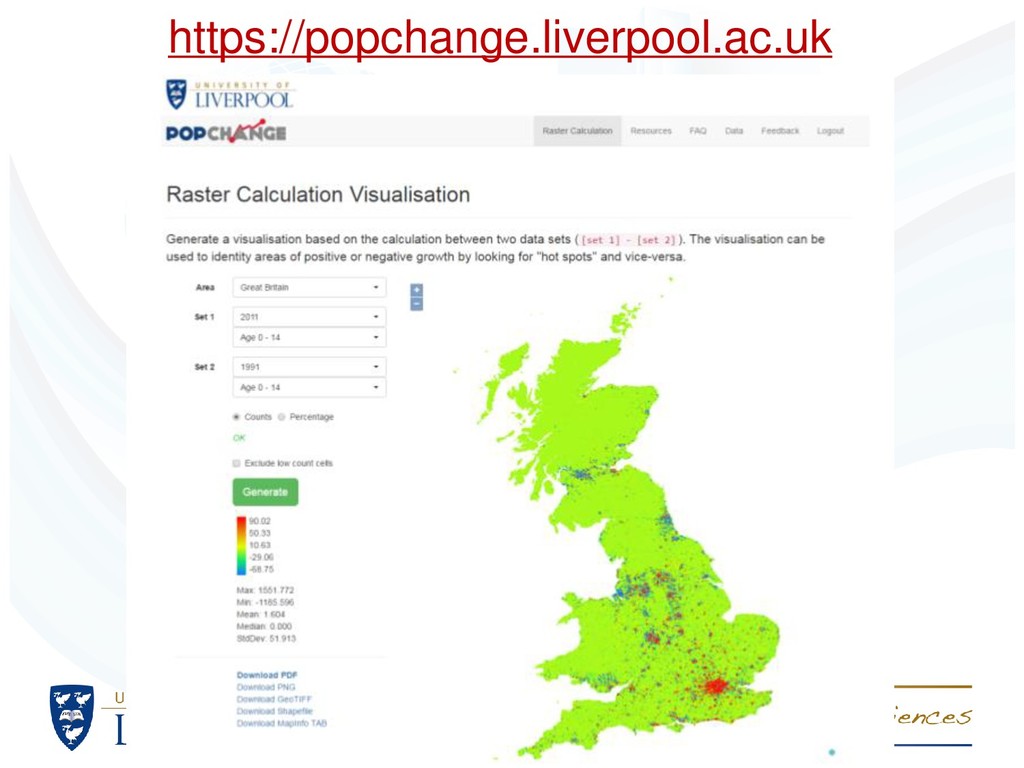
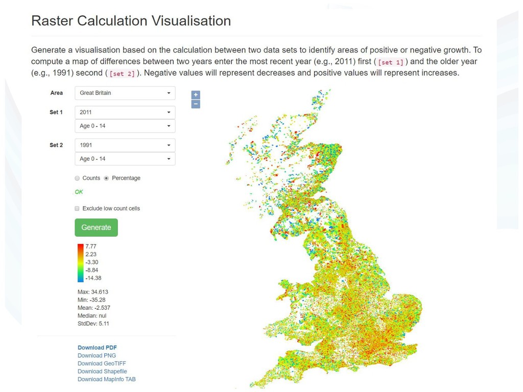
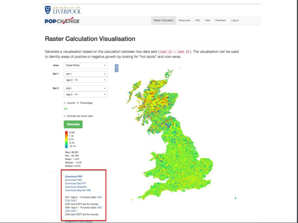
changing boundaries for small areas over time • New method of population allocation using Postcode Unit density • Web based interface for wider public participation • Code for both on GitHub
No ES/L014769/1). Team members also include Gemma Catney, Alex Singleton and Paul Williamson. The Office for National Statistics are thanked for provision of the data. Office for National Statistics, 2011 Census: Digitised Boundary Data (England and Wales) [computer file]. ESRC/JISC Census Programme, Census Geography Data Unit (UKBORDERS), EDINA (University of Edinburgh)/Census Dissemination Unit. Census output is Crown copyright and is reproduced with the permission of the Controller of HMSO and the Queen's Printer for Scotland.