Non-parametric Statistical Tests

Transcript

1. Non-parametric Statistical Tests Eskandar Alaa (ala_eskandar@comp.iust.ac.ir) Alireza Nourian (nourian@comp.iust.ac.ir)
2. Parametric Tests  Assumptions  Independence  Normality  Homoscedasticity  homogeneity of variance  e.g. T-Test 2
3. Test Case  Test Problems  5 unimodal functions  20 multimodal functions  Algorithms  PSO  IPOP-CMA-ES  CHC  SSGA  SS-arit & SS-BLX  DE-Exp & DE-Bin  SaDE 3
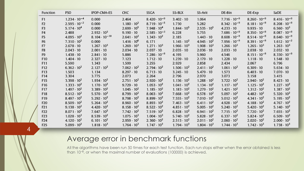
4. Average error in benchmark functions All the algorithms have been run 50 times for each test function. Each run stops either when the error obtained is less than 10−8, or when the maximal number of evaluations (100000) is achieved. 4
5. Comparisons  Pairwise comparison (1×1)  Multiple comparisons with control method (1×N)  Multiple comparisons among all methods (N×N) 5
6. Sign test (Pairwise)  H0 : Both algorithms beat each other equal times  Number of wins ~ ( 2 , 2 )  H1 : Otherwise  Z : specifies the boundary  Example  In 25 problems (Table 4)  = 0.05 ⇒ 18 wins rejects H0  = 0.1 ⇒ 17 wins rejects H0  SaDE vs. PSO  20 wins and 5 losses for SaDE ⇒ 0.95 confidence of improvement 6
7. T-Test (Parametric)  H0 : two sets of data are not significantly different from each other  Test statistic (difference of sets) follows T-Distribution  T-Distribution  Distribution of the location of the true mean, relative to the sample mean and divided by the sample standard deviation. (it’s difference) 7
8. Wilcoxon test (Pairwise)  Analogous to the Paired T-Test without Normal Distribution assumption  Do two samples represent different performances?  We just sample real algorithm performance  H0 : min(+, −) ~ Wilcoxon  + = >0 ( ) + 1 2 =0 ( )  − = <0 ( ) + 1 2 =0 ( )  Example  SaDE vs. PSO  + = 261, − = 64 ⇒ p-value = 0.00673 PSO SaDE Difference Rank 1.23e-04 8.42e-09 1.23e-04 1 2.60e-02 8.21e-09 2.59e-02 2 2.49e+00 8.09e-09 2.49e+00 3 4.10e+02 8.64e-09 4.09e+02 4 5.10e+02 1.74e+03 -1.23e+03 5 5.17e+04 6.56e+03 4.52e+04 6 + = 16, − = 5 8
9. Multiple comparisons  Multiple pairwise comparisons:  = 0 0 = 1 − 0 0 = 1 − 0 ; = 1. . − 1 0 = 1 − −1 0 0 = 1 − (1−)−1  e.g. = 0.05, k = 9 ⇒ p-value = 0.34 (terrible!) 9
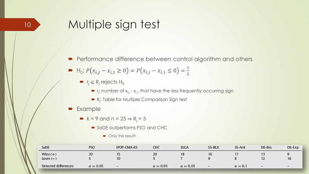
10. Multiple sign test  Performance difference between control algorithm and others  H0 : , − ,1 ≥ 0 = , − ,1 ≤ 0 = 1 2  rj ⩽ Rj rejects H0  rj : number of xi,j - xi,1 that have the less frequently occurring sign  Rj : Table for Multiple Comparison Sign test  Example  k = 9 and n = 25 ⇒ Rj = 5  SaDE outperforms PSO and CHC  Only this result! 10
11. Friedman test (1×N)  H0 : medians of the algorithms are equal  = 12 (+1) 2 − (+1)2 4  ~ −1 2 rejects H0 11
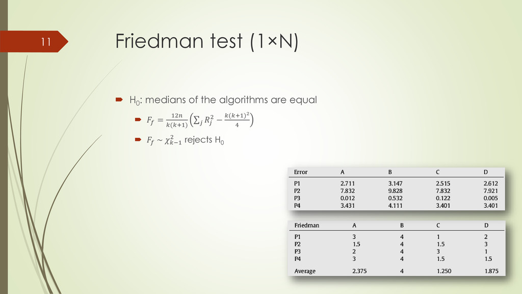
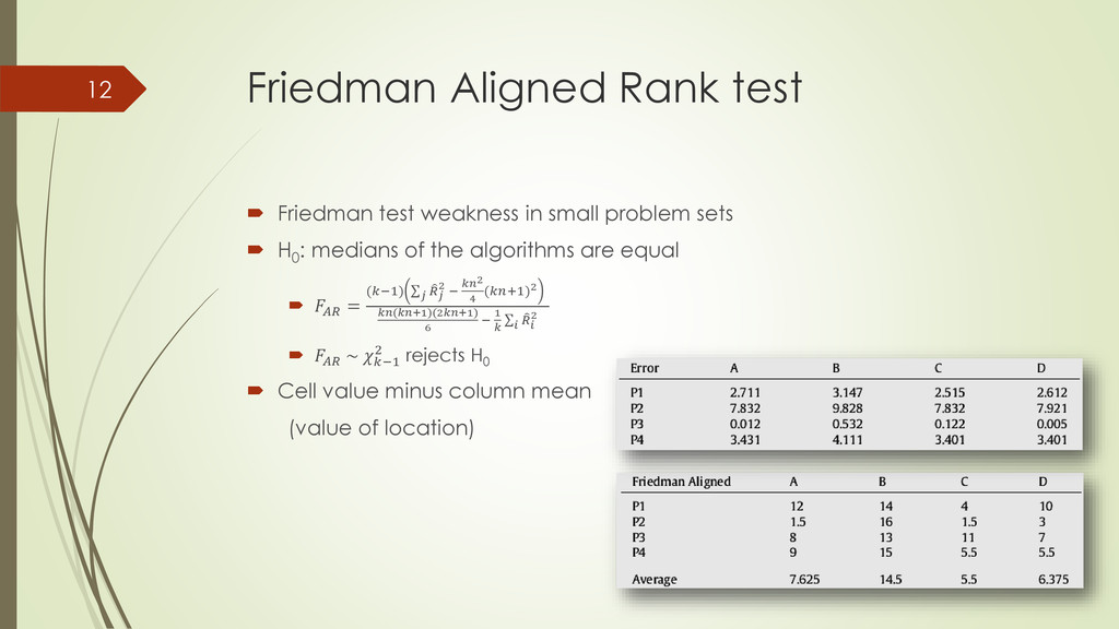
12. Friedman Aligned Rank test  Friedman test weakness in small problem sets  H0 : medians of the algorithms are equal  = (−1) 2 − 2 4 (+1)2 (+1)(2+1) 6 − 1 2  ~ −1 2 rejects H0  Cell value minus column mean (value of location) 12
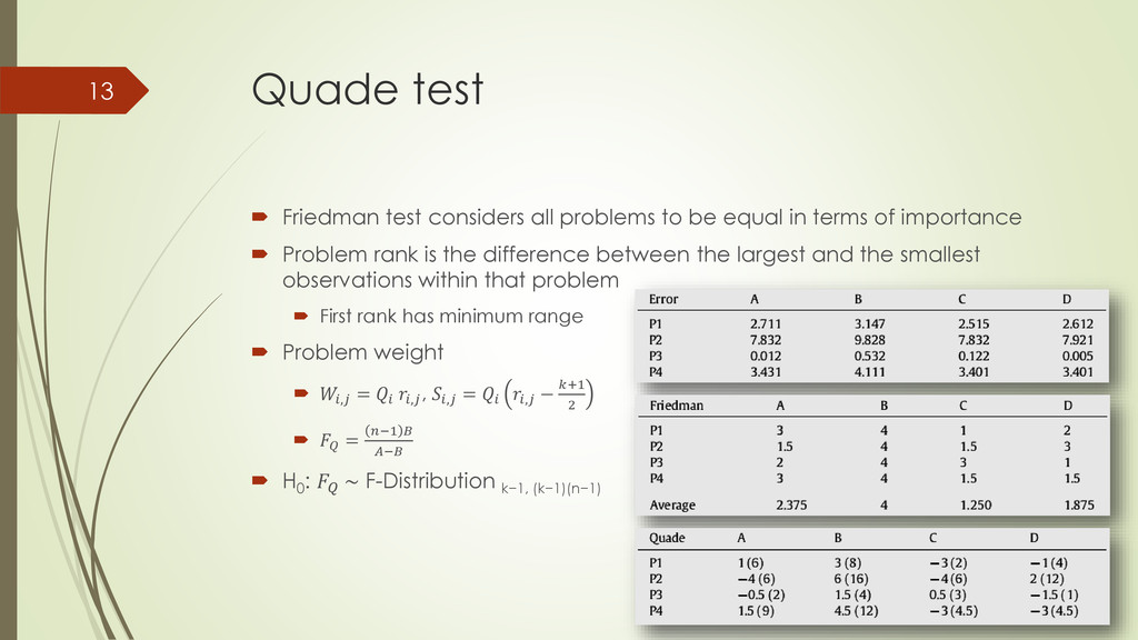
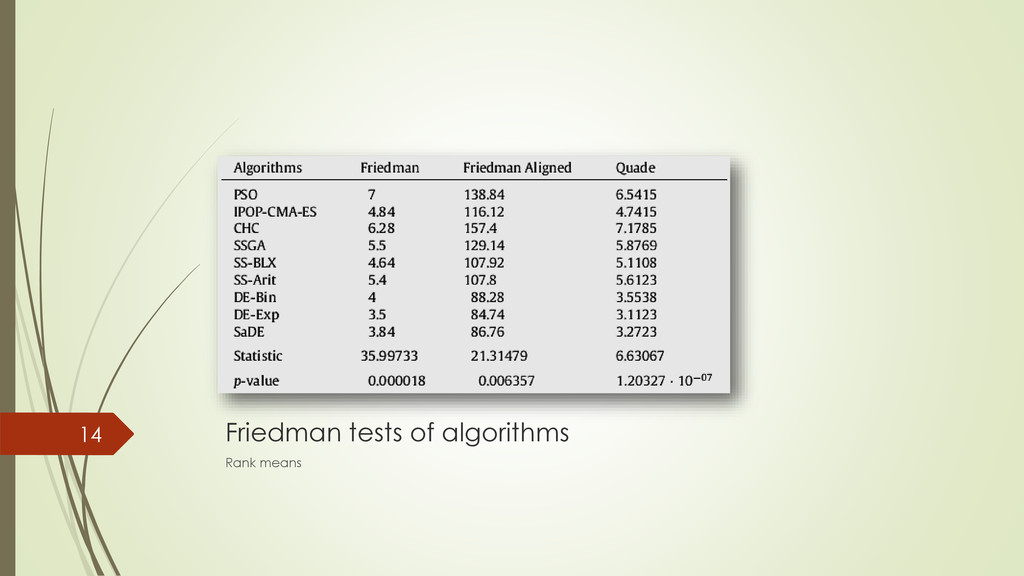
13. Quade test  Friedman test considers all problems to be equal in terms of importance  Problem rank is the difference between the largest and the smallest observations within that problem  First rank has minimum range  Problem weight  , = , , , = , − +1 2  = −1 −  H0 : ~ F-Distribution k−1, (k−1)(n−1) 13
14. Friedman tests of algorithms Rank means 14
15. Post-hoc procedures  Post-hoc test can lead to obtaining a p-value which determines the degree of rejection of each hypothesis  Unadjusted p-values  Prevent rejection of false null hypothesis  Family-wise Error Rate  ≤ 1 − (1−)−1  e.g. = 0.05, k = 9 ⇒ p-value = 0.34 15
16. Friedman test unadjusted p-values after post-hoc  Friedman  = − (+1) 6  Aligned  = − (+1) 6  Quade  − (+1)(2+1)(−1) 18(+1) 16
17. Adjustments  One-step: Benferroni = min , 1 ; = ( − 1)  Step-down: Holm = min , 1 ; = max − ∶ 1 ≤ ≤  Step-up: Hochberg = max − ∶ ≤ ≤ − 1  Two-step: Li = +1−−1  … 17
18. Contrast Estimation  Zu,v = median of performance differences between u and v  mu = Zu,v mean  estimator Mu – Mv = mu – mv  Example  SaDE best  CHC worst 18
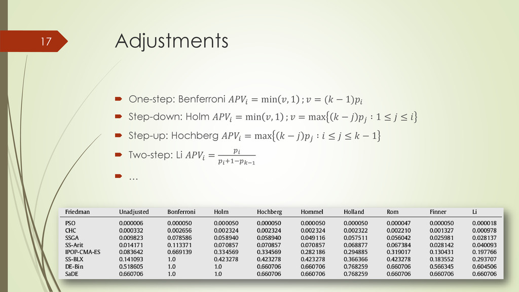
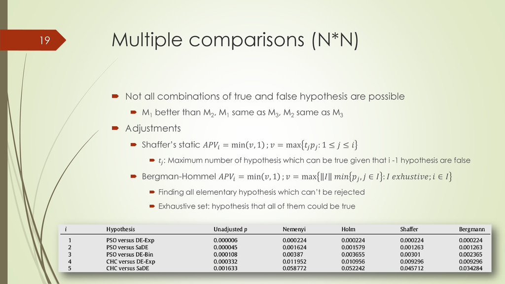
19. Multiple comparisons (N*N)  Not all combinations of true and false hypothesis are possible  M1 better than M2 , M1 same as M3 , M2 same as M3  Adjustments  Shaffer’s static = min , 1 ; = max : 1 ≤ ≤  : Maximum number of hypothesis which can be true given that i -1 hypothesis are false  Bergman-Hommel = min , 1 ; = max , ∈ : ℎ; ∈  Finding all elementary hypothesis which can’t be rejected  Exhaustive set: hypothesis that all of them could be true 19
20. Recommendations  The number of algorithms used in multiple comparisons procedures must be lower than the number of case problems  Except for Wilcoxon test  … 20
21. Conclusions  We can do better than just Average!  How many comparison are you looking for?  Pairwise comparison  Multiple comparison  Would you mind level of significance?  Sign test  Rank test  Problem difficulty  Qaude test  Taking into account relative algorithm comparisons  Post-hoc adjustments 21
22. Reference  J. Derrac, S. García, D. Molina, and F. Herrera, “A practical tutorial on the use of nonparametric statistical tests as a methodology for comparing evolutionary and swarm intelligence algorithms,” Swarm and Evolutionary Computation, vol. 1, no. 1, pp. 3–18, Mar. 2011. 22