Evaluating the Effectiveness of Illuminated and Shadowed Contour Lines

James Eynard
Bernhard Jenny
Cartography and Geovisualization Group
Oregon State University
#nacis2015

Transcript

1. Evaluating the Effectiveness of
   Illuminated and Shadowed Contour
   Lines
   James Eynard and Bernhard Jenny
   Cartography and Geovisualization Group
   Oregon State University
   NACIS | 2015 | Minneapolis, MN
   

   View Slide

2. Conventional Illuminated Shadowed
   Types of Contour Lines
   Elevation of Mt. Hood, Oregon
   

   View Slide

3. History
   Contouring Software
   User Study
   Evaluating the Effectiveness of
   Illuminated and Shadowed Contour Lines
   

   View Slide

4. 1845
   Michaelis, E.H., 1845. Passage du Splügen et de la Via Mala (map, 1:125 000) Inset in: Über die Darstellung des Hochgebirges in
   topographischen Karten. Berlin: Schropp.
   

   View Slide

5. Swiss Alpine Club, 1865. Karte der Gebirgsgruppe zwischen Lukmanier & La Greina (map 1:50 000, contour interval 30 meters, map
   by Rudolf Leuzinger)
   1865
   

   View Slide

6. Randegger, J., 188-. Wandkarte des Kantons Thurgau (map, 1:50 000). Winterthur: Topographische Anstalt von Wurster, Randegger
   & Cie.
   1880s
   

   View Slide

7. Köpcke, C., 1885. Ueber Reliefs und Relief-Photogramme. Der Civilingenieur, 31, 1–2.
   1885 – Photograph of Cardboard Cutouts
   

   View Slide

8. Pauliny, J., 1895. Mémoire über eine neue Situationspläne- und Landkarten-Darstellungsmethode. Streffleurs Österreichische
   Militärische Zeitschrift, 4 (1), 66–87.
   1891
   

   View Slide

9. Tanaka, K., 1950. The relief contour method of representing topography on maps. Geographical Review, 40 (3), 444–456.
   1950 – Tanaka Contours
   

   View Slide

10. Gilman, C.R., 1973. Photomechanical experiments in automated cartography. Journal of Research of the U.S. Geological Survey, 1
    (2), 223–228.
    1973
    

    View Slide

11. Yoeli, P. 1983. Shadowed Contours with Computer and Plotter
    1983 – Computer-based techniques
    

    View Slide

12. Eyton, J. R. 1984. Raster contouring. Geo-Processing 2: 221-42.
    1984 – Computer-based techniques
    

    View Slide

13. Kennelly, P. and Kimerling, A. J. (2001). ‘Modifications of Tanaka’s illuminated contour method’, Cartography and Geographic
    Information Science, 28, pp. 111–123.
    2001 – Modified Tanaka Contour Lines
    

    View Slide

14. Imhof, E. (1965). Kartographische Geländedarstellung. Walter de Gruyter.
    Imhof, E. (2007). Cartographic relief presentation. ESRI, Inc..
    

    View Slide

15. View Slide

16. Manual and Semi-automated Techniques
    •  Time consuming, inconsistent results
    •  Calligraphy-style pens
    •  Digital
    –  Adobe Illustrator,
    Photoshop
    –  Scripts
    

    View Slide

17. Contouring Software
    

    View Slide

18. Generalization of Contour Lines
    

    View Slide

19. Adjust Illumination Angle
    NW
    SE
    

    View Slide

20. Adjust Contour Interval
    100 m 300 m
    

    View Slide

21. Adjust Line Thickness
    

    View Slide

22. Adjust Line Thickness
    (for illuminated and shadowed side)
    

    View Slide

23. Adjust Transition Angle
    90º 120º
    

    View Slide

24. Despeckle
    

    View Slide

25. Minimum Distance Between Contour Lines
    

    View Slide

26. Shadowed Contour Lines
    

    View Slide

27. View Slide

28. User Study
    

    View Slide

29. Previous User Studies
    Several studies on contour map interpretation, but…
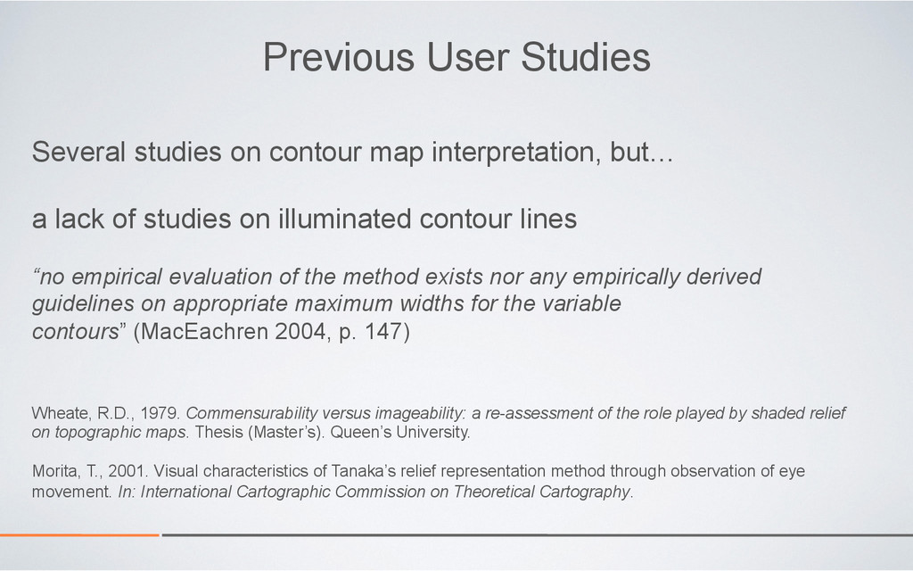
    a lack of studies on illuminated contour lines
    “no empirical evaluation of the method exists nor any empirically derived
    guidelines on appropriate maximum widths for the variable
    contours” (MacEachren 2004, p. 147)
    Wheate, R.D., 1979. Commensurability versus imageability: a re-assessment of the role played by shaded relief
    on topographic maps. Thesis (Master’s). Queen’s University.
    Morita, T., 2001. Visual characteristics of Tanaka’s relief representation method through observation of eye
    movement. In: International Cartographic Commission on Theoretical Cartography.
    

    View Slide

30. User Study Hypothesis
    Certain features of topography can be interpreted
    more quickly and accurately by map-readers with
    illuminated and shadowed contours maps than with
    conventional contour maps.
    

    View Slide

31. User Study
    •  Conventional contour lines
    •  Shadowed contour lines
    •  Illuminated contour lines
    •  Shaded relief
    Within Groups
    Mechanical Turk -> Qualtrics, 397 participants
    

    View Slide

32. User Study Sections
    Tutorial
    Relative Height Questions
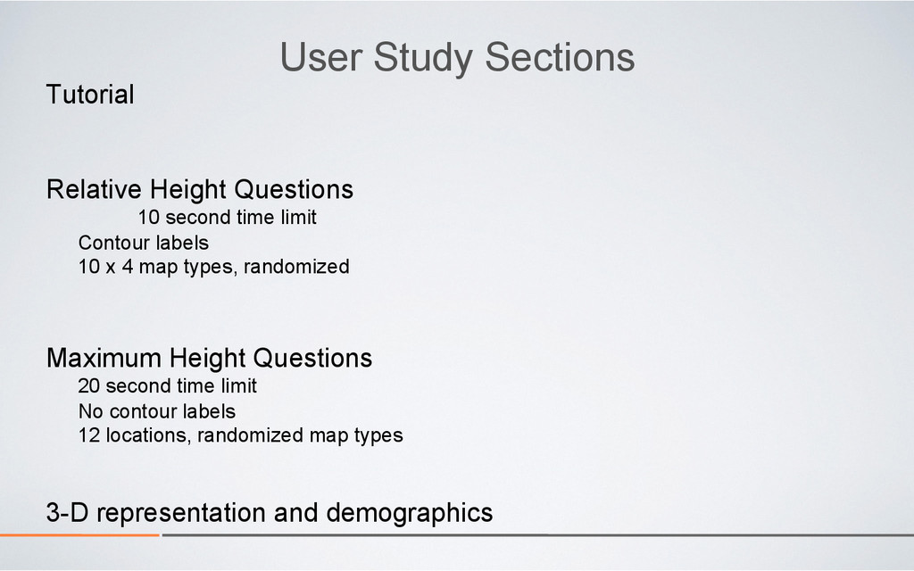
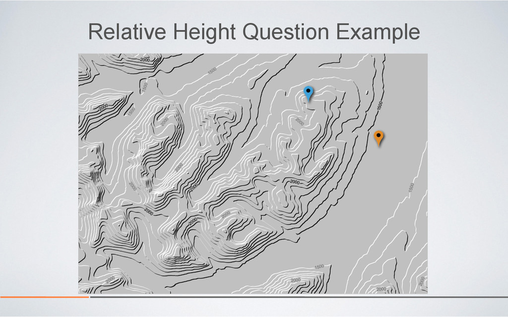
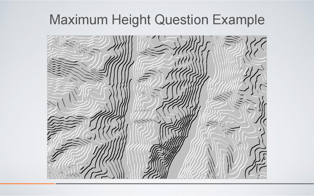
    10 second time limit
    Contour labels
    10 x 4 map types, randomized
    Maximum Height Questions
    20 second time limit
    No contour labels
    12 locations, randomized map types
    3-D representation and demographics
    

    View Slide

33. Relative Height Question Example
    

    View Slide

34. Maximum Height Question Example
    

    View Slide

35. User Study Results
    •  Relative Height Question
    •  Accuracy
    •  Timing
    •  Maximum Height Question
    •  Accuracy
    •  Timing
    •  3-D representation and demographics
    

    View Slide

36. User Study Results
    Relative Height Question – Accuracy
    Map$type$pairs$ χ2$ Sig$
    ! ! !
    Illuminated!–!shadowed! 4.6750! yes!
    Illuminated!–!conventional! 10.0831! yes!
    Illuminated!–!shaded!relief! 15.2345! yes!
    Shadowed!–!conventional! 1.0151! no!
    Shadowed!–!shaded!relief! 3.0127! no!
    Shaded!relief!–!conventional! 0.5214! no!
    ! ! !
    !
    McNemar’s test results, χ2-crit = 3.8415
    89.4%&
    84.8%&
    81.5%&
    83.1%&
    50%&
    60%&
    70%&
    80%&
    90%&
    100%&
    Illuminated& Shadowed& Shaded&
    Relief&
    Conven?onal&
    Percent'Correct'
    

    View Slide

37. User Study Results
    Relative Height Question – Timing
    Map$type$
    Mean$timing$
    (seconds)$
    Std$dev$
    timing$
    !
    !
    !
    Illuminated! 3.0! 1.3!
    Shadowed! 3.4! 1.5!
    Conventional! 3.6! 1.6!
    Shaded!relief! 2.5! 1.1!
    ! ! !
    !
    Wilcoxon signed-ranks test – Significance for all map pairs at p < 0.01
    Map$type$pairs$ Effect$r$ Effect$size$sig$
    ! ! !
    Illuminated!–!shadowed! 0.23! low!
    Illuminated!–!conventional! 0.30! med!
    Illuminated!–!shaded!relief! 0.34! med!
    Shadowed!–!conventional! 0.12! low!
    Shadowed!–!shaded!relief! 0.46! med!
    Shaded!relief!–!conventional! 0.49! med!
    ! ! !
    !
    

    View Slide

38. User Study Results
    Maximum Height Question – Accuracy
    Map$type$ Mean$accuracy$ Std$dev$
    ! !
    !
    Illuminated,!unlabeled! 79.5%! 15.7%!
    Shadowed,!unlabeled! 75.3%! 20.8%!
    Conventional,!labeled! 79.4%! 18.1%!
    Shaded!relief! 69.6%! 19.8%!
    ! ! !
    !
    Wilcoxon signed-ranks test and Cohen’s r effect size results
    Map$type$pairs$ P,value$ Sig$ Effect$r$ Effect$size$sig$
    ! ! ! ! !
    Illuminated!–!shadowed! Illuminated!–!conventional! 0.741! no! X! X!
    Illuminated!–!relief! Shadowed!–!conventional! Shadowed!–!shaded!relief! Shaded!relief!–!conventional! ! ! ! ! !
    !
    

    View Slide

39. User Study Results
    Maximum Height Question – Timing
    Map$type$
    Mean$timing$
    (seconds)$
    Std$dev$
    timing$
    !
    !
    !
    Illuminated,!unlabeled! 6.2! 3.6!
    Shadowed,!unlabeled! 6.1! 3.7!
    Conventional,!labeled! 6.3! 3.3!
    Shaded!relief! 7.9! 3.8!
    ! ! !
    !
    

    View Slide

40. For each map type, participants were asked if they
    agree with the following statement:
    This map shows variations in elevation well and
    produces an appearance of the third dimension.
    43.1%&
    25.3%&
    8.9%&
    7.1%&
    43.1%&
    57.5%&
    45.7%&
    30.8%&
    5.6%&
    8.2%&
    20.2%&
    19.3%&
    6.6%&
    7.4%&
    22.4%&
    35.4%&
    0%& 10%& 20%& 30%& 40%& 50%& 60%& 70%& 80%& 90%& 100%&
    Relief&
    Illuminated&
    Shadowed&
    Conven@onal&
    Strongly&Agree& Agree& Neither& Disagree& Strongly&Disagree&
    

    View Slide

41. User Study Results
    Demographics
    No significance
    •  Age
    •  Gender
    •  Education level
    •  Self-evaluated topographic map reading ability
    

    View Slide

42. Conclusions
    Illuminated contour lines – quicker and more accurate
    Shadowed contour lines – quicker and more accurate to a lesser
    extent for some map reading tasks
    Mechanical Turk – unexpected results
    

    View Slide

43. Limitations and Potential Use
    •  Neutral background
    •  Bathymetry maps
    •  Other statistical surfaces
    •  Variations and future user studies
    •  Subtle color and line width changes
    •  More detailed maps
    •  Various scales
    

    View Slide

44. View Slide

45. Created by Sam Hooper and published in the Atlas of Polar Regions
    

    View Slide

46. Created by Mathias Wigum and Bernhard Jenny and published in the Atlas of Polar Regions
    

    View Slide

47. Acknowledgements
    Oregon State University
    Tom Patterson
    Dr. Richard Oliver
    AAG Cartography Specialty Group
    Bojan Šavrič, Charles Preppernau, Brooke Marston, and Lawrence Sim
    

    View Slide

48. Pyramid Shader – free and open source
    software for creating illuminated and
    shadowed contour lines
    •  Shaded relief
    •  Plan oblique relief
    •  Hypsometric colors
    •  Local hypsometric colors
    •  Terrain generalization
    •  Bivariate colors
    •  Slope
    •  Aspect
    

    View Slide

49. View Slide

50. Pyramid Shader
    www.terraincartography.com/PyramidShader
    Questions?
    

    View Slide