FOSS4G NA | Interacting with National Water Model (NWM) Predictions

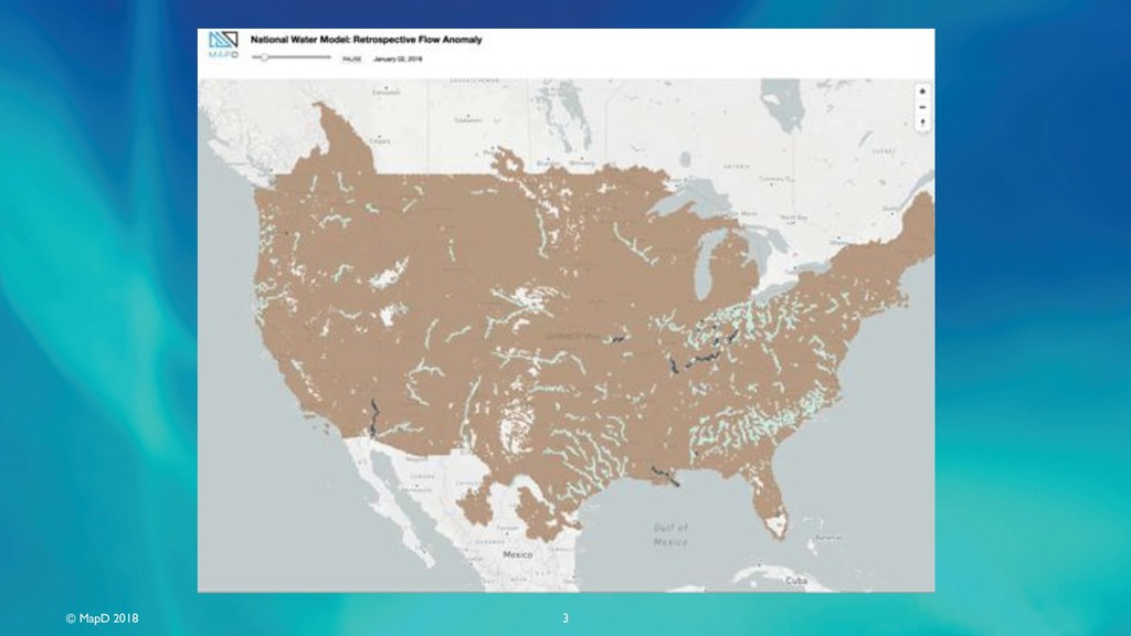
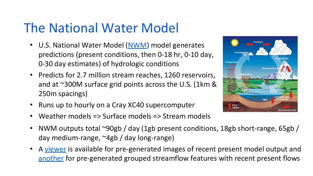
The increasing availability of large-scale cloud computing resources has enabled large-scale environmental predictive models such as the National Water Model (NWM) to be run essentially continuously. Such models generate so many predictions that the output alone presents a big data computing challenge to interact with and learn from.

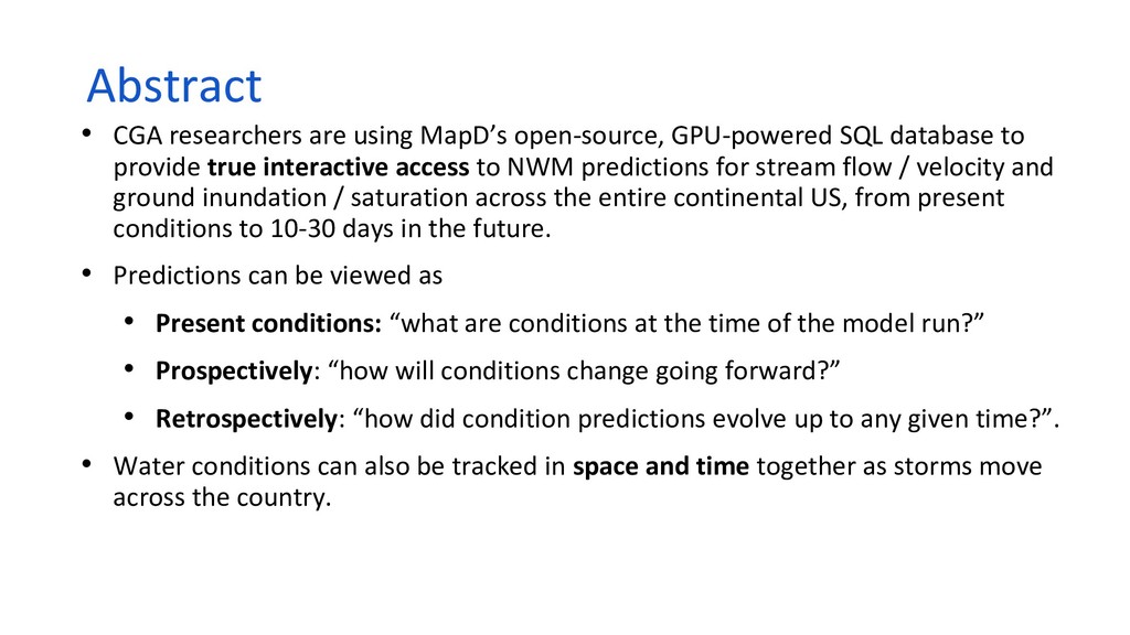
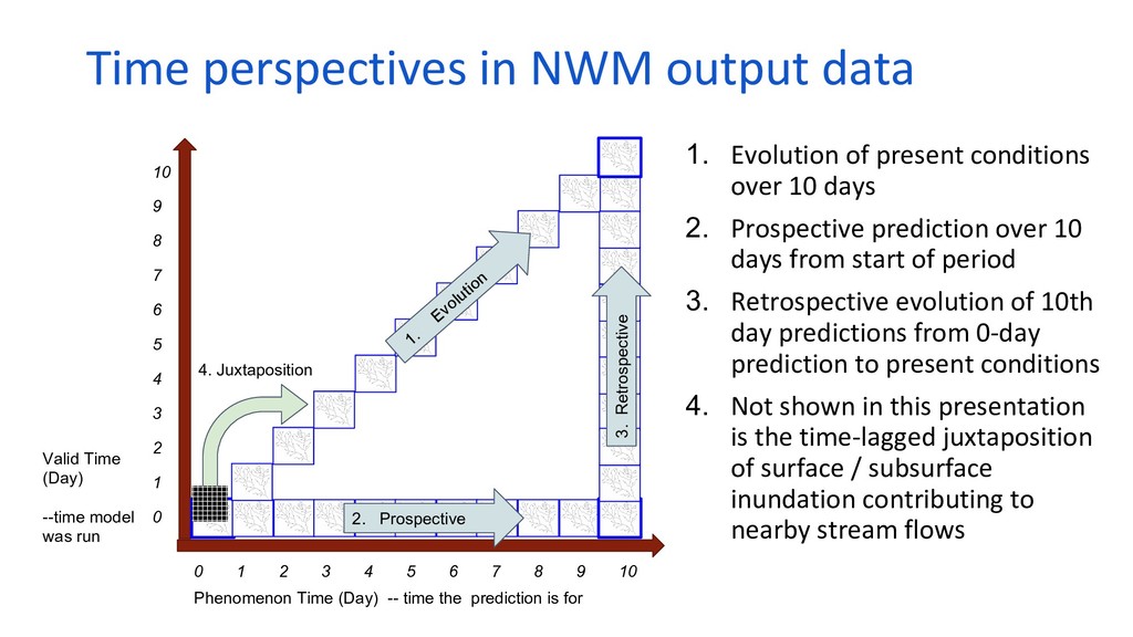
Researchers at the Harvard Center for Geographic Analysis are working with the open-source, GPU-powered database MapD to provide true interactive access to NWM predictions for stream flow and ground saturation across the entire continental US and from present conditions to 18 days in the future. Predictions can be viewed prospectively, “how will conditions change going forward?” as well as retrospectively, “how did condition predictions evolve up to any given present?”. Water conditions can also be tracked in space and time together as storms move across the country.

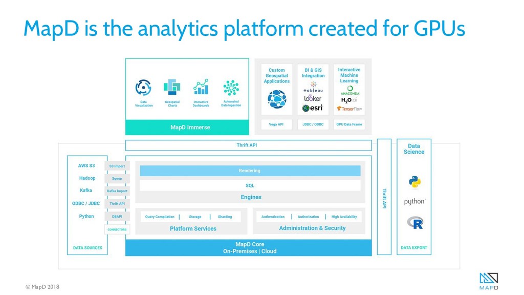
The speed and flexibility of the GPU analytics platform allows questions such as “how did the stream flow prediction error change over time?" to be answered quickly with SQL queries, and facilitates joining in additional data such as the location of bridges and other vulnerable infrastructure, all with relatively low-cost computing resources. MapD and other open-source high-performance geospatial computing tools have the potential to greatly broaden access to the full benefits of large-scale environmental models being deployed today.

Transcript

1. © MapD 2018 Interacting with National Water Model (NWM) Predictions Josh Lieberman & Aaron Williams May 15, 2018
2. © MapD 2018 Introductions Aaron Williams VP of Global Community @_arw_ aaron@mapd.com /in/aaronwilliams/ /williamsaaron Josh Lieberman Senior Research Scientist @lieberjosh jlieberman@fas.harvard.edu /in/joshua-lieberman-ab81262/ /lieberjosh slides: https://speakerdeck.com/mapd/
3. © MapD 2018 © MapD 2018 3 ANIMATION
4. Core Density Makes a Huge Difference 4 GPU Processing CPU Processing 40,000 Cores 20 Cores *fictitious example Latency Throughput CPU 1 ns per task (1 task/ns) x (20 cores) = 20 tasks/ns GPU 10 ns per task (0.1 task per ns) x (40,000 cores) = 4,000 task per ns Latency: Time to do a task. | Throughput: Number of tasks per unit time.
5. © MapD 2018 MapD is the analytics platform created for GPUs
6. © MapD 2018 And Now … Native Geospatial! 6 First Data Types • POINT • LINE • POLYGON First Functions • DISTANCE • CONTAINS Get Involved • Roadmap Being Discussed MapD (OSS) Working Group geo-wg@mapd.com • Beta Available Now Email Aaron - aaron@mapd.com
7. © MapD 2018 Advanced memory management Three-tier caching to GPU RAM for speed and to SSDs for persistent storage 7 SSD or NVRAM STORAGE (L ) GB to TB - GB/sec CPU RAM (L ) GB to TB - GB/sec GPU RAM (L ) GB to GB - GB/sec Hot Data Speedup = x to x Over Cold Data Warm Data Speedup = x to x Over Cold Data Cold Data COMPUTE LAYER STORAGE LAYER Data Lake/Data Warehouse/System Of Record
8. © MapD 2018 The GPU Open Analytics Initiative Creating common data frameworks to accelerate data science on GPUs 8 /mapd/pymapd /gpuopenanalytics/pygdf
9. © MapD 2018 © MapD 2018 • Catch up with us at FOSS4G! Visit our table any time to see our latest demos Tue 2pm MapD CEO: Speed Meets Scale Tue 2:45pm Florida LIDAR data in MapD Thurs 2-5pm MapD for Analysts Workshop • github.com/mapd OSS repo • mapd.cloud Get a MapD instance in less than 60 seconds • community.mapd.com Ask questions and share your experiences 9 Next Steps
10. © MapD 2018 Thank you! Any questions? Aaron Williams VP of Global Community @_arw_ aaron@mapd.com /in/aaronwilliams/ /williamsaaron Josh Lieberman Senior Research Scientist @ jlieberman@fas.harvard.edu /in/joshua-lieberman-ab81262/ /lieberjosh slides: https://speakerdeck.com/mapd/
11. Using MapD’s GPU-powered SQL Database to Interact with National Water Model (NWM) Predictions Aaron Williams, MapD Technologies Josh Lieberman, Harvard Center for Geographic Analysis (CGA) Devika Kakkar, CGA Benjamin Lewis , CGA FOSS4G North America May 14, 2018 to May 17, 2018
12. Using MapD’s GPU-powered SQL Database to Interact with National Water Model (NWM) Predictions Aaron Williams, MapD Technologies Devika Kakkar, Harvard Center for Geographic Analysis (CGA) Josh Lieberman, Harvard Center for Geographic Analysis (CGA) Benjamin Lewis , Harvard Center for Geographic Analysis (CGA) Boston Data Visualization and MapD Meetup April 25, 2018
13. Abstract • CGA researchers are using MapD’s open-source, GPU-powered SQL database to provide true interactive access to NWM predictions for stream flow / velocity and ground inundation / saturation across the entire continental US, from present conditions to 10-30 days in the future. • Predictions can be viewed as • Present conditions: “what are conditions at the time of the model run?” • Prospectively: “how will conditions change going forward?” • Retrospectively: “how did condition predictions evolve up to any given time?”. • Water conditions can also be tracked in space and time together as storms move across the country.
14. Workshop Outline • The National Water Model (NWM) • Time perspective in NWM • Current work with NWM and MapD • Amazon MapD AMI • Data Flow from NWM to MapD • Table optimization • Database switches and memory • Visualization in Map D • Streamflow Perspectives: Present, Prospective, Retrospective • Streamflow aggregate by county • Ground Inundation grid (Texas)
15. “Big” geospatial data: as few as a million features • Most sets of geographic features are modest: thousands to millions in size. But... • Increasing spatial resolution is changing this: e.g. National Hydro Datasets Medium Res -> ~3M reaches, High Res -> ~30M reaches. Similar for gridded data, e.g. 10m DEM -> 1m Lidar-based 3DEP increases volume 100x. • Time is changing this: multiple observations and predictions for multiple feature properties quickly combine into billions of records. • Traditional GIS software struggles to access and visualize, let alone analyze such scales and structures of datasets. • Datasets with 1-100 billion records are becoming common in academic, business, and government domains.
16. Model Simulation and Prediction Data • Most observation data is already “model-based” and uses a computational “procedure” to convert a measurement of a “stimulus” into an estimation of an “observed property” for a “feature of interest” (O&M model, SOSA/SSN ontology) -----> • Simulation and prediction models extend this same paradigm to generate properties at places and/or times that differ from those at which measurements are made. • Model outputs are characterized by at least 3 different time senses: a. Valid Time - the time or time interval within which the model inputs apply and the output is therefore valid. b. Phenomenon Time - the time of the observed / simulated / predicted property estimate c. Result Time - the time at which model output is available for use (may be some time after the Valid Time for lengthy computations). Feature of Interest Property Of Observed Property Estim ates Result Yields Observation @ vt, pt, rt Stimulus M easures Used In Sensor Executed In Procedure
17. High performance model interpretation • Computing needs are at the scale of the volume, velocity, and variety of the model output and other data to be processed, juxtaposed, or compared. • Needs may also vary according to the specific hypotheses to be tested, methods to be employed, and the number of interpreters working with a given model output. • Parallel computing can address volume but may not produce the throughput to support interactive interpretation nor be cost effective to scale for many users. • GPU-based computing can increase throughput through efficient “parallelism in place” with fast execution of certain operations on thousands of inexpensive processor cores, if the data fit into GPU memory. • Specific computational components assembled into tool chains provide flexibility for evolving model analysis and visualization needs.
18. The National Water Model • U.S. National Water Model (NWM) model generates predictions (present conditions, then 0-18 hr, 0-10 day, 0-30 day estimates) of hydrologic conditions • Predicts for 2.7 million stream reaches, 1260 reservoirs, and at ~300M surface grid points across the U.S. (1km & 250m spacings) • Runs up to hourly on a Cray XC40 supercomputer • Weather models => Surface models => Stream models • NWM outputs total ~90gb / day (1gb present conditions, 18gb short-range, 65gb / day medium-range, ~4gb / day long-range) • A viewer is available for pre-generated images of recent present model output and another for pre-generated grouped streamflow features with recent present flows
19. Time perspectives in NWM output data 1. Evolution of present conditions over 10 days 2. Prospective prediction over 10 days from start of period 3. Retrospective evolution of 10th day predictions from 0-day prediction to present conditions 4. Not shown in this presentation is the time-lagged juxtaposition of surface / subsurface inundation contributing to nearby stream flows Phenomenon Time (Day) -- time the prediction is for Valid Time (Day) --time model was run 0 1 2 3 4 5 6 7 8 9 10 10 9 8 7 6 5 4 3 2 1 0 1. Evolution 2. Prospective 3. Retrospective 4. Juxtaposition
20. Current work with NWM and MapD • Develop data download, storage, database loading procedures • Configure and install MapD on 1-GPU EC2 instances • Load nationwide stream reach mid-points and 1km (down-sampled from 250m to fit in GPU memory) grid point geometries to MapD store. • Load stream flow / velocity and soil inundation / saturation outputs for once-daily present conditions and 1-10 day predictions over a 10-day period at the beginning of 2018. Learn virtues of pandas dataframe. • Construct SQL views and tables to join stream and point locations with model output values. Discover that (some) views work differently than equivalent queries in MapD. • Develop dashboard views in MapD Immerse to visualize the results. Learn hidden tricks, GPU utilities, and undocumented configuration switches.
21. Amazon MapD AMI
22. Data Flow from NWM to MapD • Harvesting o NWM output files in NetCDF format downloaded from website / ftpsite. • Storage o 2-month test dataset at 6-hour intervals of present and predicted conditions stored in AWS S3. o Next: a rolling 1-2 month time window of datafiles to be maintained on the MOC • Preprocessing / loading to MapD o NetCDF -> Xarray -> Pandas Dataframe -> PyMapD -> MapD table o Geometric coordinates stored separately from model output parameters • Limitations o Data are initially loaded onto disk, then column-wise into CPU and/or GPU memory for query and/or rendering (1 K-80 GPU -> ~11gb data memory)
23. Data Flow from NWM to MapD Geo • Preprocessing / loading to MapD o NetCDF -> Xarray ( N-dimensional variants of the core pandas data structures) o Xarray -> Pandas dataframe o Add geometry column to the dataframe using shapely o ...Geometric coordinates stored separately from model output parameters o Convert data frame to geodataframe with geopanda o Export geodataframe to shapefile with geopanda / fiona o Import shapefile to MapD: • COPY streams FROM '...MyGeometries.shp' WITH (geo='true'); o
24. Table optimization in MapD • MapD is a column-oriented full-scan relational database without indexes • It manages data on disk and loads table columns as needed into CPU and/or GPU memory • GPU memory is generally more limited than CPU memory, so it is important to size and number of the data columns used for visualization • Both the number and length of columns to be queried, e.g. in a map, should be carefully planned to fit into GPU memory • Large datasets may be loaded into MapD, then a subset queried to create smaller working columns that fit into GPU memory for faster operation Scale/performance
25. Database switches and memory • Issues with views that have joins (exception) versus tables created from joins (success): create view | table channel_flow_anomaly as select a.feature_id, b.longitude, b.latitude, (a.streamflow - b.avgflow) as anomflow, a.valid_time as vtime, a.phenomenon_time as ptime from nwm_channel a join channel_coord_avg b on a.feature_id=b.feature_id; Exception: Query couldn’t keep the entire working set of columns in GPU memory • The following switches were added to mapd.conf to optimize the memory usage: • enable-watchdog = false: Tries to predict whether a query will fit into GPU memory and stops it if that doesn’t appear to be the case • allow-cpu-retry = true: Allows queries that do not fit in the GPU’s available memory to fall back and be executed on the CPU if appropriate • Other tips and advice sprinkled throughout MapD Community Forum
26. Present - Prospective - Retrospective http://52.168.111.218:8080/ http://52.168.111.218:8081/ http://52.168.111.218:8082
27. Visualizing perspectives 1-3 on MapD and Immerse
28. Zooming in
29. Aggregation by County Chloropleth Map
30. Ground inundation grid (Texas)
31. Next Steps • Rolling 2-month current NWM model output store • Deployment on OpenShift in Mass Open Cloud • Nationwide land surface outputs • Spatial operations to analyze water impacts on people and infrastructure • Visualization of model sequencing (weather -> land -> waterbodies) • Work with historical data for Hurricane Harvey, e.g. NWM <-> imagery comparisons • User applications for flood / high-water notifications • Other datasets of interest (nationwide air pollution, voter affiliation)
32. Conclusions • Interpretation of simulation / prediction model outputs for geographic entities can be a big data challenge that is both significant and separate from that of running the models. Without adequate tools to interpret this scale of data, the usefulness of creating and running the models themselves is reduced. • GPU-based data analysis and visualization tools such as MapD offer good possibilities for addressing this challenge with fast data interaction, cost effective deployment, and flexible integration with other tools. • DBMS’ such as MapD still require significant expertise to use effectively when “pushing the envelope” on new capabilities. • CGA has learned much already from working with MapD and NWM model outputs and plan to apply this to other use cases and domains.
33. Resources • More notes on the Project Wiki https://github.com/cga-harvard/HPC_on_MOC/ • MapD Core code https://github.com/mapd/mapd-core • Collaboration announcements http://gis.harvard.edu/announcements/renewed-collaboration-bet ween-cga-and-mapd-accelerate-research-gpus
34. Thank You