Visualizing Geospatial Data on GPUs with MapD

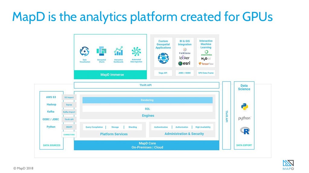
There has been an explosion of geospatial data sources and collection in recent years, and with it the need for technologies that data analysts can use to query and visualize those very large data sets interactively, exploring and taking action on the data in real-time. In this hands-on tutorial, each attendee will be given a geospatial data set to work with, which they will use to ingest into MapD. By the end of this workshop, you'll learn how to query extremely large geospatial data and visualize it.

In this workshop, participants will be given access to a MapD instance, and hand-on instruction in the following:

-How to install and setup the MapD platform in the cloud, or on prem.
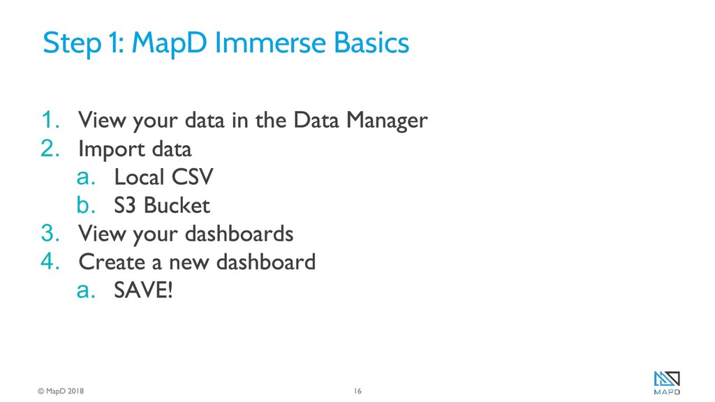
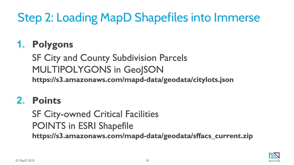
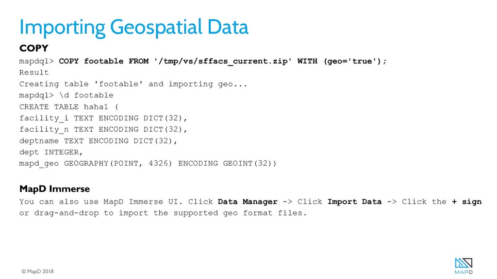
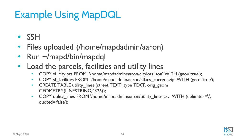
-How to import a geospatial dataset, either one of our samples or one of your own.
-How to create dashboards with geospatial charts in MapD Immerse.
-How to create multi-layer maps, combining data from multiple sources.
-How to update dashboards and share them.

Transcript

3. Agenda • • •
4. Do This Now 1. 2. 3.
6. MapD is the analytics platform created for GPUs
7. DEMO
8. Advanced memory management SSD or NVRAM STORAGE (L3) 250GB to 20TB 1-2 GB/sec CPU RAM (L2) 32GB to 3TB 70-120 GB/sec GPU RAM (L1) 24GB to 256GB 1000-6000 GB/sec Hot Data Speedup = 1500x to 5000x Over Cold Data Warm Data Speedup = 35x to 120x Over Cold Data Cold Data COMPUTE LAYER STORAGE LAYER Data Lake/Data Warehouse/System Of Record
9. MapD Core: Query Compilation with LLVM
10. MapD Immerse: Hybrid Rendering
11. Categories of common MapD use cases Operational Analytics • Thwart Banking Fraud • Scan for Cyber Threats • Fine-tune Advertising • Maintain the Utility Grid Geospatial Analytics • Monitor Networks • Ready Logistics • Forecast Micro-weather Data Science • Model Financial Markets • Predict Maintenance • Predict Staffing Levels
12. The GPU Open Analytics Initiative (GOAI)
13. • • ML Examples
14. Tutorial A: Importing Geospatial Data into MapD Cloud
15. Last Chance ... 1. 2. 3.
16. Step 1: MapD Immerse Basics 1. 2. a. b. 3. 4. a.
17. Geospatial Objects Type POINT A point described by two coordinates. LINESTRING A sequence of 2 or more points and the lines that connect them. POLYGON A set of one or more rings (closed line strings), with the first representing the shape (external ring) and the rest representing holes in that shape (internal rings) MULTIPOLYGON A set of one or more polygons.
18. Step 2: Loading MapD Shapefiles into Immerse 1. 2.
19. Tutorial B: Importing and Rendering with the MapD API & Vega
20. Geospatial Table It’s now possible to create tables with geospatial columns CREATE TABLE geo1 ( p1 POINT, l1 LINESTRING, poly1 POLYGON, mpoly1 MULTIPOLYGON); By default, geospatial objects are created as geometries (planar spatial data types). Type definition can be extended to include the spatial reference identification (SRID) and compression mode information. CREATE TABLE geo2 ( p2 GEOMETRY(POINT), l2 GEOMETRY(LINESTRING, 900913), poly2 GEOMETRY(POLYGON, 4326) ENCODING NONE, mpoly2 GEOMETRY(MULTIPOLYGON, 4326) ENCODING GEOINT(32));
21. Geospatial Table mapdql> CREATE TABLE geo (pz POINT, p POINT, l LINESTRING) WITH (fragment_size=2); mapdql> \d geo CREATE TABLE geo ( pz GEOMETRY(POINT), p GEOMETRY(POINT), l GEOMETRY(LINESTRING)) WITH (FRAGMENT_SIZE = 2)
22. Importing Geospatial Data One way is through INSERT, using WKT string values: mapdql> \d geo CREATE TABLE geo ( p POINT, l LINESTRING, poly POLYGON) mapdql> insert into geo values('POINT(20 20)', 'LINESTRING(40 0, 40 40)', 'POLYGON(( 0 0, 40 0, 40 40, 0 40, 0 0 ))'); The COPY command is the fastest option for importing geospatial data, and binary shape files and GEOJSON files at this time. COPY table_name FROM full_path WITH (Geo=‘True’)
23. Importing Geospatial Data mapdql> COPY footable FROM '/tmp/vs/sffacs_current.zip' WITH (geo='true'); Result Creating table 'footable' and importing geo... mapdql> \d footable CREATE TABLE haha1 ( facility_i TEXT ENCODING DICT(32), facility_n TEXT ENCODING DICT(32), deptname TEXT ENCODING DICT(32), dept INTEGER, mapd_geo GEOGRAPHY(POINT, 4326) ENCODING GEOINT(32)) You can also use MapD Immerse UI. Click Data Manager -> Click Import Data -> Click the + sign or drag-and-drop to import the supported geo format files.
24. Example Using MapDQL • • • • • • • •
25. Geospatial Functions ST_GeomFromText Return a specified geometry from Well-Known Text representation (WKT) ST_GeogFromText Return a specified geography from Well-Known Text representation (WKT)
26. Geospatial Functions ST_Transform Return a new geometry with its coordinates transformed to a different spatial reference. The only supported transform in this release is WGS84 to Web Mercator, e.g. ST_Transform(ST_GeogFromText('POINT(-71.064544 42.28787)',4326),900913) ST_SetSRID Set the SRID on a geometry to a particular integer value.
27. Geospatial Functions ST_XMin Returns X minima of a geometry. ST_XMax Returns X maxima of a geometry. ST_YMin Returns Y minima of a geometry. ST_YMax Returns Y maxima of a geometry. ST_StartPoint Returns the first point of a LINESTRING as a POINT. ST_EndPoint Returns the last point of a LINESTRING as a POINT. ST_PointN Return the Nth point of a LINESTRING as a POINT. ST_SRID Returns the spatial reference identifier for the underlying object
28. Geospatial Functions ST_Distance Returns shortest planar distance between geometries. Returns shortest geodesic distance between geographies (in meters, limited support). ST_Contains Returns true if first geometry contains the second one.
29. Geospatial Rendering with Vega/MapBoxGL JS • git clone https://github.com/omveda/mapd-vega-mapboxgl-geo • Follow the instructions in the README to install software on your laptop. ❏ cd mapd-vega-mapboxgl-geo ❏ yarn install ❏ npm start MapD Vega is based on the open-source Vega Specification, it has been adapted to drive the rendering engine directly on the result set of a SQL query without ever requiring the data to leave the GPU. The MapD Connector API makes it easy to send the Vega JSON to the backend, which renders the visualization and returns a base64-encoded PNG image to the client. A Vega specification includes: • a data property that specifies and filters data source(s). • a marks property that defines the basic visualization graphic of a data item. • a scales property that defines geometry or applies additional attributes to the data item visualization. • viewing area dimensions.
30. Load Using MapDQL • • • • • • • •
31. • • • • Next Steps
32. Thank you! Questions?