Introduction to R for Genomic Data Analysis

【第2回】ゼロから始めるゲノム解析（R編）

Transcript

1. ゲノム解析のためのR入門 【第2回】ゼロから始めるゲノム解析 2020 年 9 月 25 日 onouyek@Bioinformatics Tokyo
2. 目的 データ分析の手順を理解してもらい、ゲノム解析に必要なRプログラミングの基本を 習得します。
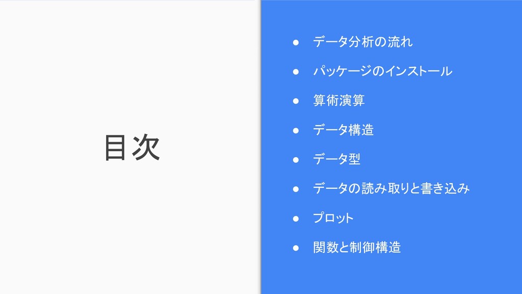
3. 目次 • データ分析の流れ • パッケージのインストール • 算術演算 • データ構造 • データ型 • データの読み取りと書き込み • プロット • 関数と制御構造
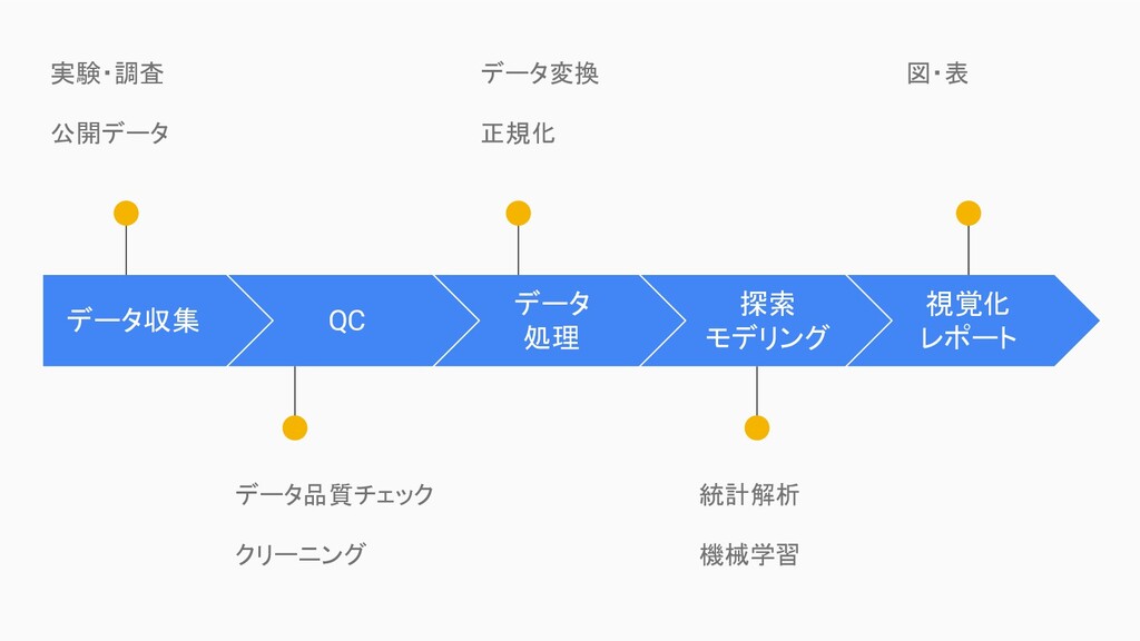
4. データ分析の流れ
5. データ収集 実験・調査 公開データ QC データ品質チェック クリーニング データ 処理 データ変換 正規化 探索 モデリング 統計解析 機械学習 視覚化 レポート 図・表
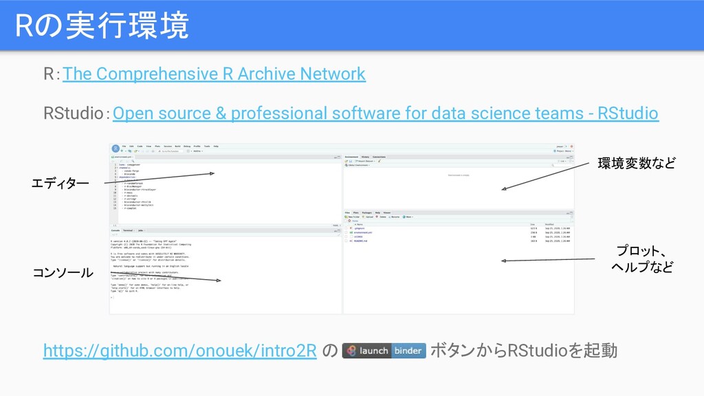
6. R：The Comprehensive R Archive Network RStudio：Open source & professional software for data science teams - RStudio https://github.com/onouek/intro2R の ボタンからRStudioを起動 Rの実行環境 エディター コンソール 環境変数など プロット、 ヘルプなど
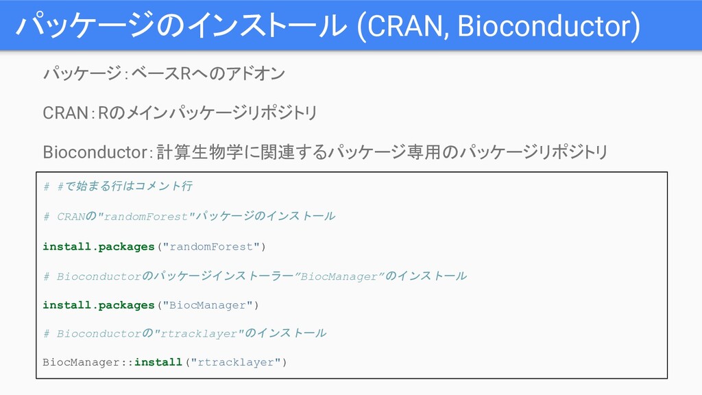
7. パッケージのインストール (CRAN, Bioconductor) パッケージ：ベースRへのアドオン CRAN：Rのメインパッケージリポジトリ Bioconductor：計算生物学に関連するパッケージ専用のパッケージリポジトリ # #で始まる行はコメント行 # CRANの"randomForest"パッケージのインストール install.packages("randomForest") # Bioconductorのパッケージインストーラー”BiocManager”のインストール install.packages("BiocManager") # Bioconductorの"rtracklayer"のインストール BiocManager::install("rtracklayer")
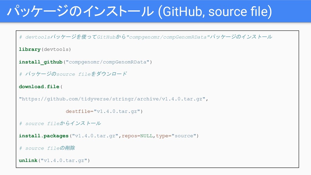
8. パッケージのインストール (GitHub, source file) # devtoolsパッケージを使ってGitHubから"compgenomr/compGenomRData"パッケージのインストール library(devtools) install_github("compgenomr/compGenomRData") # パッケージのsource fileをダウンロード download.file( "https://github.com/tidyverse/stringr/archive/v1.4.0.tar.gz", destfile="v1.4.0.tar.gz") # source fileからインストール install.packages("v1.4.0.tar.gz",repos=NULL,type="source") # source fileの削除 unlink("v1.4.0.tar.gz")
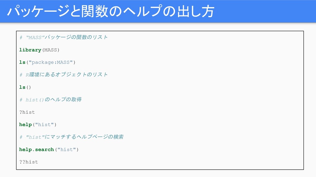
9. パッケージと関数のヘルプの出し方 # “MASS”パッケージの関数のリスト library(MASS) ls("package:MASS") # R環境にあるオブジェクトのリスト ls() # hist()のヘルプの取得 ?hist help("hist") # "hist"にマッチするヘルプページの検索 help.search("hist") ??hist
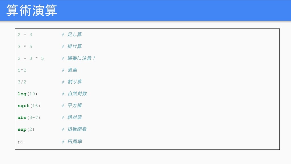
10. 算術演算 2 + 3 # 足し算 3 * 5 # 掛け算 2 + 3 * 5 # 順番に注意！ 5^2 # 累乗 3/2 # 割り算 log(10) # 自然対数 sqrt(16) # 平方根 abs(3-7) # 絶対値 exp(2) # 指数関数 pi # 円周率
11. データ構造
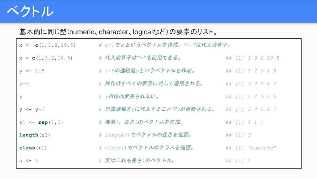
12. ベクトル 基本的に同じ型（numeric、character、logicalなど）の要素のリスト。 x <- c(1,3,2,10,5) # c()でｘというベクトルを作成。”<-”は代入演算子。 x = c(1,3,2,10,5) # 代入演算子は”=”も使用できる。 ## [1] 1 3 2 10 5 y <- 1:5 # 1~5の連続値yというベクトルを作成。 ## [1] 1 2 3 4 5 y+2 # 操作はすべての要素に対して適用される。 ## [1] 3 4 5 6 7 y # y自体は変更されない。 ## [1] 1 2 3 4 5 y <- y+2 # 計算結果をyに代入することでyが更新される。 ## [1] 3 4 5 6 7 r1 <- rep(1,3) # 要素1、長さ3のベクトルを作成。 ## [1] 1 1 1 length(r1) # length()でベクトルの長さを確認。 ## [1] 3 class(r1) # class()でベクトルのクラスを確認。 ## [1] “numeric” a <- 1 # 実はこれも長さ1のベクトル。 ## [1] 1
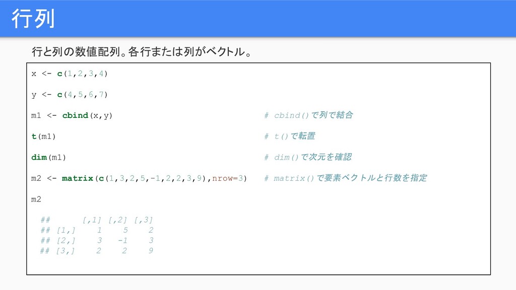
13. 行列 行と列の数値配列。各行または列がベクトル。 x <- c(1,2,3,4) y <- c(4,5,6,7) m1 <- cbind(x,y) # cbind()で列で結合 t(m1) # t()で転置 dim(m1) # dim()で次元を確認 m2 <- matrix(c(1,3,2,5,-1,2,2,3,9),nrow=3) # matrix()で要素ベクトルと行数を指定 m2 ## [,1] [,2] [,3] ## [1,] 1 5 2 ## [2,] 3 -1 3 ## [3,] 2 2 9
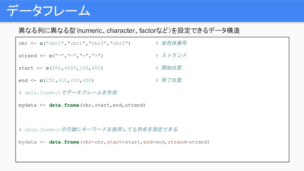
14. データフレーム 異なる列に異なる型（numeric、character、factorなど）を設定できるデータ構造 chr <- c("chr1","chr1","chr2","chr2") # 染色体番号 strand <- c("-","-","+","+") # ストランド start <- c(200,4000,100,400) # 開始位置 end <- c(250,410,200,450) # 終了位置 # data.frame()でデータフレームを作成 mydata <- data.frame(chr,start,end,strand) # data.frame()の引数にキーワードを使用しても列名を指定できる mydata <- data.frame(chr=chr,start=start,end=end,strand=strand)
15. データフレームの要素の抽出 列番号または名前で特定の列を抽出したり、行番号で特定の行を抽出したりできる。 mydata[,2:4] # 列番号2,3,4の列を抽出 mydata[,c("chr","start")] # 列名がchrとstartの列を抽出 mydata$start # 列名がstartの列を抽出 mydata[c(1,3),] # 行番号1,3の行を抽出 mydata[mydata$start>400,] # start列が400以上の行を抽出
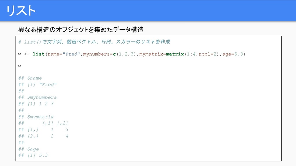
16. リスト 異なる構造のオブジェクトを集めたデータ構造 # list()で文字列、数値ベクトル、行列、スカラーのリストを作成 w <- list(name="Fred",mynumbers=c(1,2,3),mymatrix=matrix(1:4,ncol=2),age=5.3) w ## $name ## [1] "Fred" ## ## $mynumbers ## [1] 1 2 3 ## ## $mymatrix ## [,1] [,2] ## [1,] 1 3 ## [2,] 2 4 ## ## $age ## [1] 5.3
17. リストの要素の抽出 位置または名前を二重括弧で指定して抽出できる。 # 位置（3番目）を指定してオブジェクトを抽出 w[[3]] ## [,1] [,2] ## [1,] 1 3 ## [2,] 2 4 # 名前（mynumbers）を指定してオブジェクトを抽出 w[["mynumbers"]] ## [1] 1 2 3 # 名前（age）を$で指定してオブジェクトを抽出 w$age ## [1] 5.3
18. ファクター カテゴリーデータを格納するためのデータ構造 ※data.frame()でデータフレームを作成した場合に、文字列はデフォルトでファクターとして格納される。 features=c("promoter","exon","intron") f.feat=factor(features) # factor()関数でf.featにカテゴリーデータを格納 f.feat ## [1] promoter exon intron ## Levels: exon intron promoter
19. データ型 Rの4つのデータ型（numeric、logical、character、integer） # numericベクトルxを作成 x <- c(1,3,2,10,5) ## [1] 1 3 2 10 5 # logicalベクトルxを作成 x <- c(TRUE,FALSE,TRUE) ## [1] TRUE FALSE TRUE # characterベクトルxを作成 x <- c("sds","sd","as") ## [1] "sds" "sd" "as" class(x) ## [1] "character" # integerベクトルxを作成 x <- c(1L,2L,3L) ## [1] 1 2 3 class(x) ## [1] “integer”
20. データの読み取りと書き込み
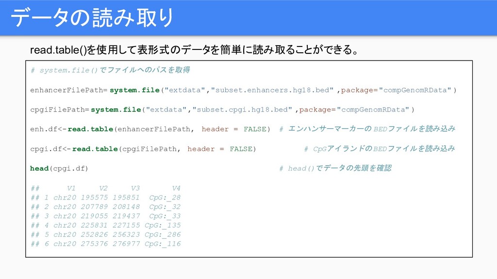
21. read.table()を使用して表形式のデータを簡単に読み取ることができる。 データの読み取り # system.file()でファイルへのパスを取得 enhancerFilePath= system.file("extdata","subset.enhancers.hg18.bed" ,package="compGenomRData" ) cpgiFilePath= system.file("extdata","subset.cpgi.hg18.bed" ,package="compGenomRData" ) enh.df<-read.table(enhancerFilePath, header = FALSE) # エンハンサーマーカーの BEDファイルを読み込み cpgi.df<-read.table(cpgiFilePath, header = FALSE) # CpGアイランドのBEDファイルを読み込み head(cpgi.df) # head()でデータの先頭を確認 ## V1 V2 V3 V4 ## 1 chr20 195575 195851 CpG:_28 ## 2 chr20 207789 208148 CpG:_32 ## 3 chr20 219055 219437 CpG:_33 ## 4 chr20 225831 227155 CpG:_135 ## 5 chr20 252826 256323 CpG:_286 ## 6 chr20 275376 276977 CpG:_116
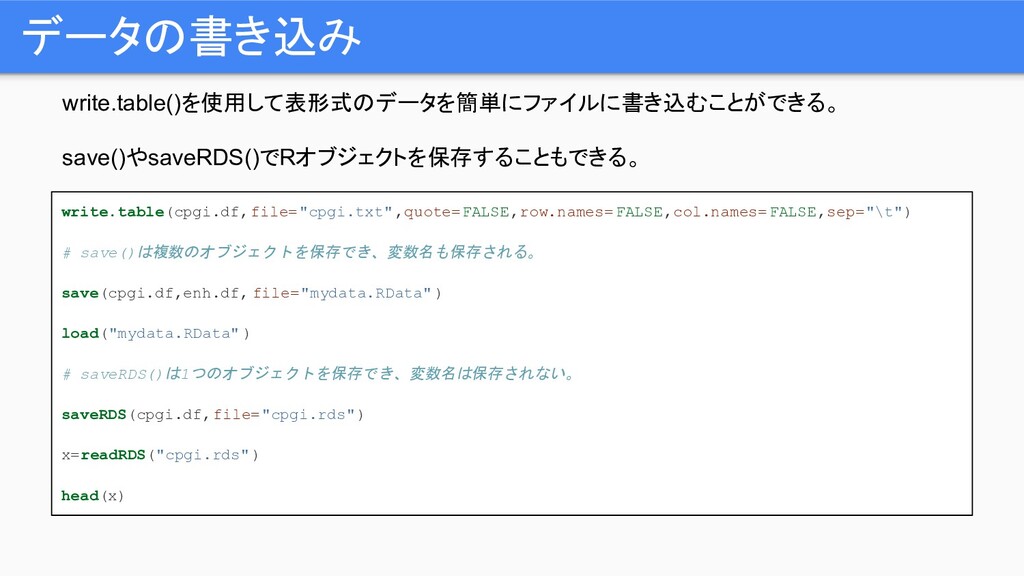
22. write.table()を使用して表形式のデータを簡単にファイルに書き込むことができる。 save()やsaveRDS()でRオブジェクトを保存することもできる。 データの書き込み write.table(cpgi.df,file="cpgi.txt",quote=FALSE,row.names=FALSE,col.names=FALSE,sep="\t") # save()は複数のオブジェクトを保存でき、変数名も保存される。 save(cpgi.df,enh.df, file="mydata.RData" ) load("mydata.RData" ) # saveRDS()は1つのオブジェクトを保存でき、変数名は保存されない。 saveRDS(cpgi.df,file="cpgi.rds") x=readRDS("cpgi.rds") head(x)
23. プロット
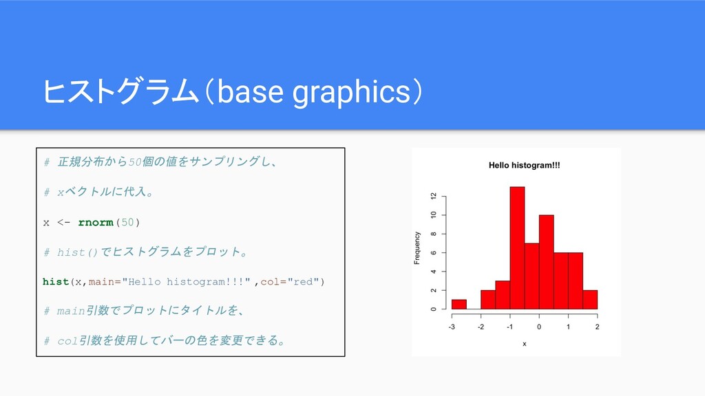
24. ヒストグラム（base graphics） # 正規分布から50個の値をサンプリングし、 # xベクトルに代入。 x <- rnorm(50) # hist()でヒストグラムをプロット。 hist(x,main="Hello histogram!!!" ,col="red") # main引数でプロットにタイトルを、 # col引数を使用してバーの色を変更できる。
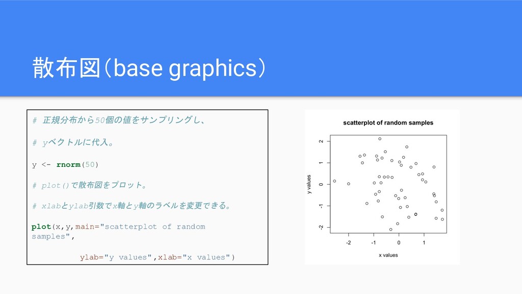
25. 散布図（base graphics） # 正規分布から50個の値をサンプリングし、 # yベクトルに代入。 y <- rnorm(50) # plot()で散布図をプロット。 # xlabとylab引数でx軸とy軸のラベルを変更できる。 plot(x,y,main="scatterplot of random samples", ylab="y values",xlab="x values")
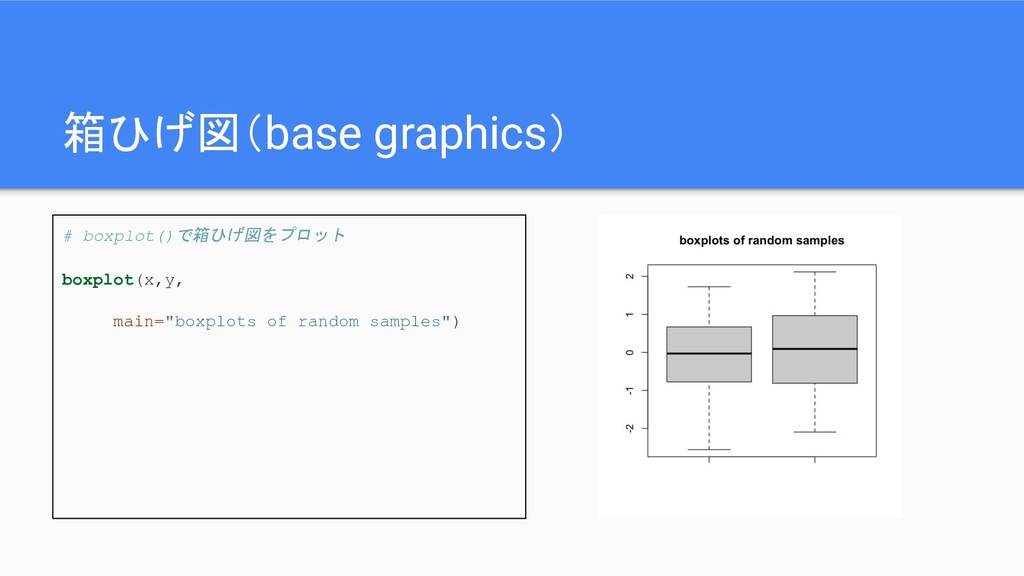
26. 箱ひげ図（base graphics） # boxplot()で箱ひげ図をプロット boxplot(x,y, main="boxplots of random samples")
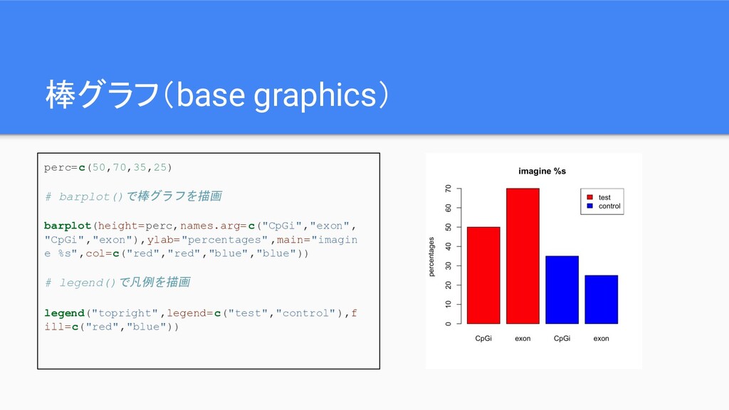
27. 棒グラフ（base graphics） perc=c(50,70,35,25) # barplot()で棒グラフを描画 barplot(height=perc,names.arg=c("CpGi","exon", "CpGi","exon"),ylab="percentages" ,main="imagin e %s",col=c("red","red","blue","blue")) # legend()で凡例を描画 legend("topright",legend=c("test","control"),f ill=c("red","blue"))
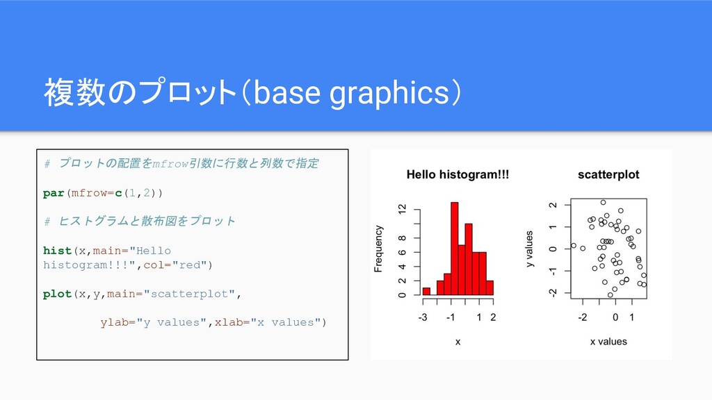
28. 複数のプロット（base graphics） # プロットの配置をmfrow引数に行数と列数で指定 par(mfrow=c(1,2)) # ヒストグラムと散布図をプロット hist(x,main="Hello histogram!!!",col="red") plot(x,y,main="scatterplot", ylab="y values",xlab="x values")
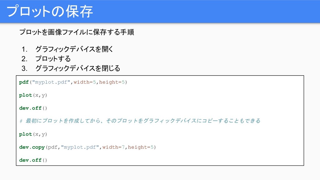
29. プロットを画像ファイルに保存する手順 1. グラフィックデバイスを開く 2. プロットする 3. グラフィックデバイスを閉じる プロットの保存 pdf("myplot.pdf",width=5,height=5) plot(x,y) dev.off() # 最初にプロットを作成してから、そのプロットをグラフィックデバイスにコピーすることもできる plot(x,y) dev.copy(pdf,"myplot.pdf",width=7,height=5) dev.off()
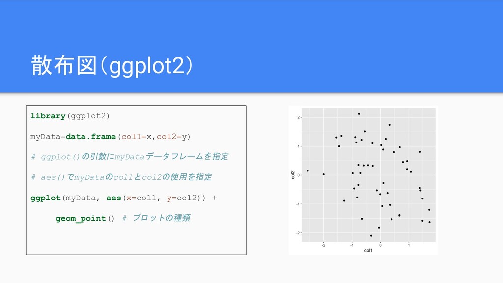
30. 散布図（ggplot2） library(ggplot2) myData=data.frame(col1=x,col2=y) # ggplot()の引数にmyDataデータフレームを指定 # aes()でmyDataのcol1とcol2の使用を指定 ggplot(myData, aes(x=col1, y=col2)) + geom_point() # プロットの種類
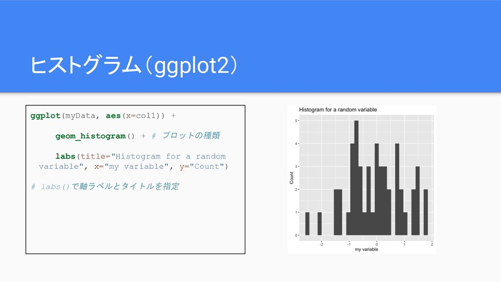
31. ヒストグラム（ggplot2） ggplot(myData, aes(x=col1)) + geom_histogram() + # プロットの種類 labs(title="Histogram for a random variable", x="my variable", y="Count") # labs()で軸ラベルとタイトルを指定
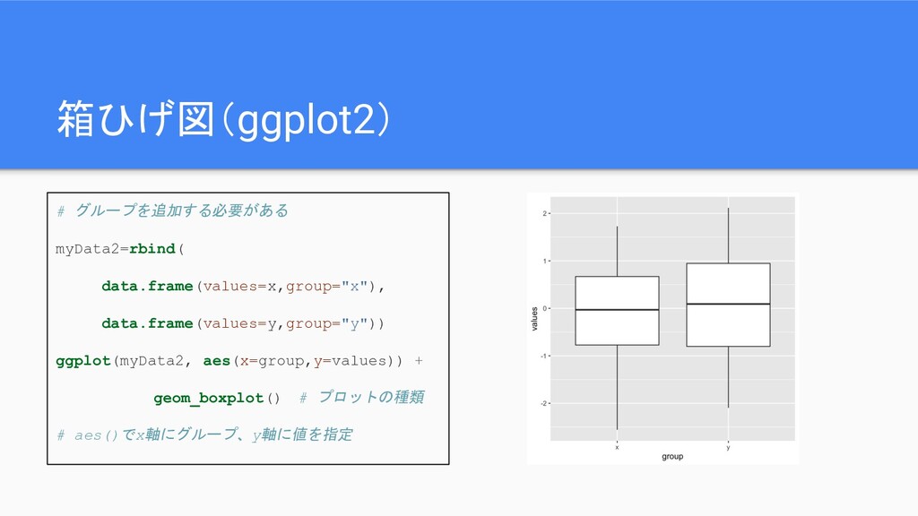
32. 箱ひげ図（ggplot2） # グループを追加する必要がある myData2=rbind( data.frame(values=x,group="x"), data.frame(values=y,group="y")) ggplot(myData2, aes(x=group,y=values)) + geom_boxplot()　# プロットの種類 # aes()でx軸にグループ、y軸に値を指定
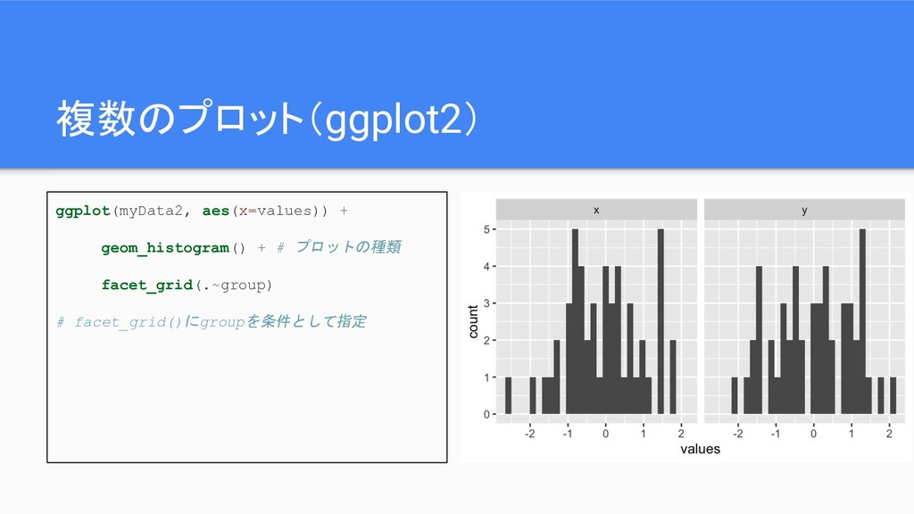
33. 複数のプロット（ggplot2） ggplot(myData2, aes(x=values)) + geom_histogram() + # プロットの種類 facet_grid(.~group) # facet_grid()にgroupを条件として指定
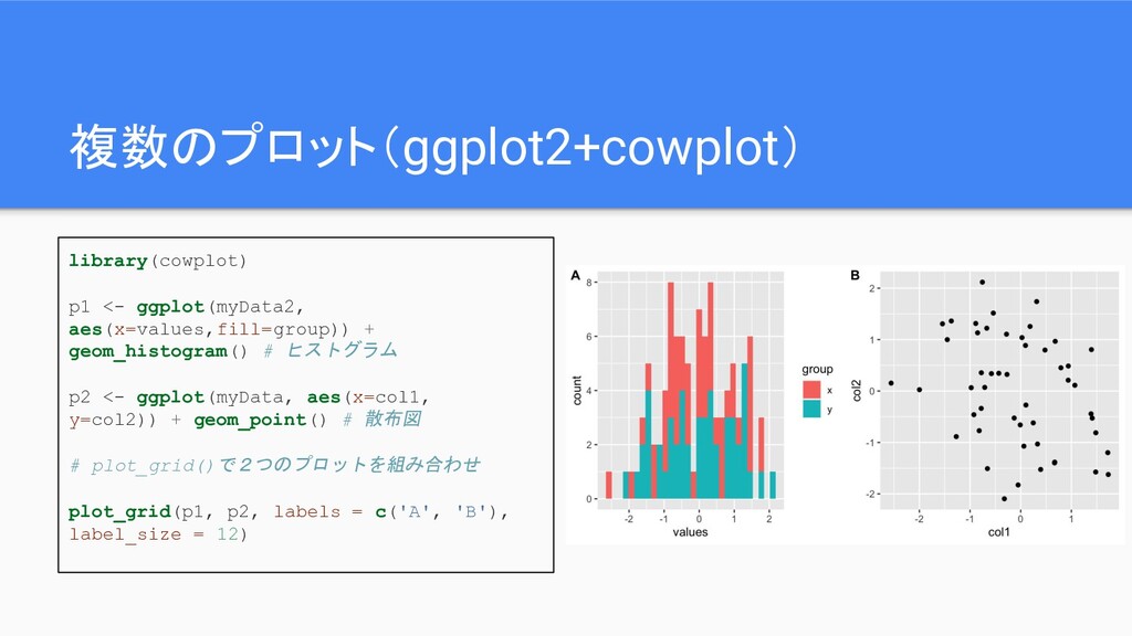
34. 複数のプロット（ggplot2+cowplot） library(cowplot) p1 <- ggplot(myData2,　 aes(x=values,fill=group)) + geom_histogram() # ヒストグラム p2 <- ggplot(myData, aes(x=col1, y=col2)) + geom_point() # 散布図 # plot_grid()で２つのプロットを組み合わせ plot_grid(p1, p2, labels = c('A', 'B'), label_size = 12)
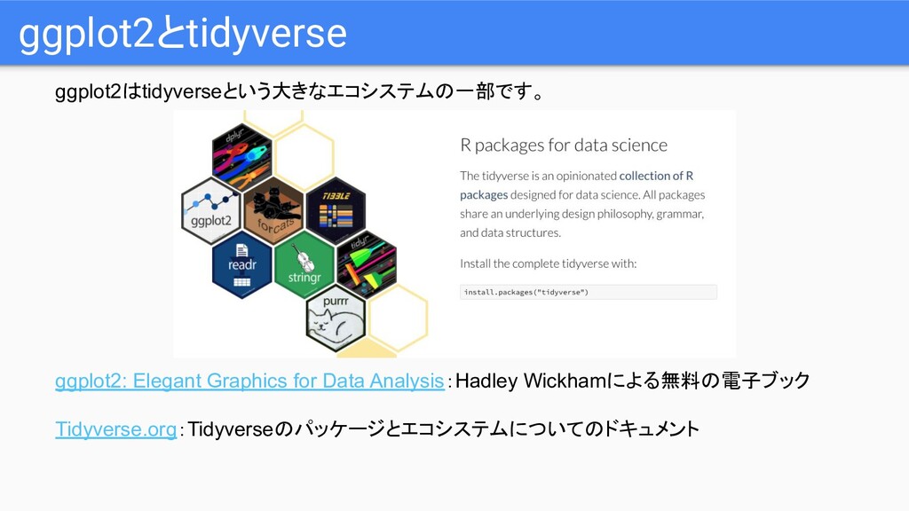
35. ggplot2とtidyverse ggplot2はtidyverseという大きなエコシステムの一部です。 ggplot2: Elegant Graphics for Data Analysis：Hadley Wickhamによる無料の電子ブック Tidyverse.org：Tidyverseのパッケージとエコシステムについてのドキュメント
36. 関数と制御構造
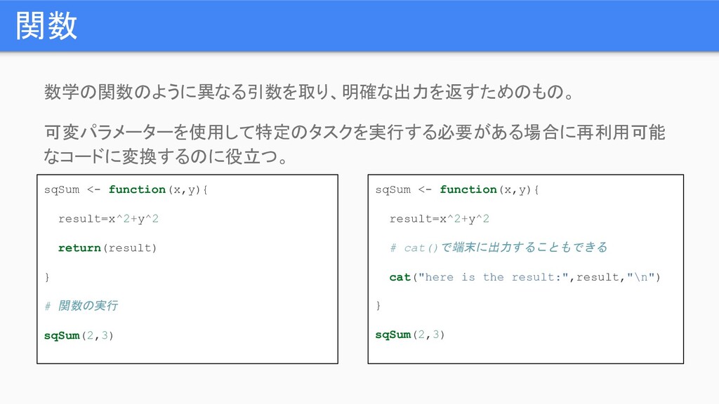
37. 関数 数学の関数のように異なる引数を取り、明確な出力を返すためのもの。 可変パラメーターを使用して特定のタスクを実行する必要がある場合に再利用可能 なコードに変換するのに役立つ。 sqSum <- function(x,y){ result=x^2+y^2 return(result) } # 関数の実行 sqSum(2,3) sqSum <- function(x,y){ result=x^2+y^2 # cat()で端末に出力することもできる cat("here is the result:",result,"\n") } sqSum(2,3)
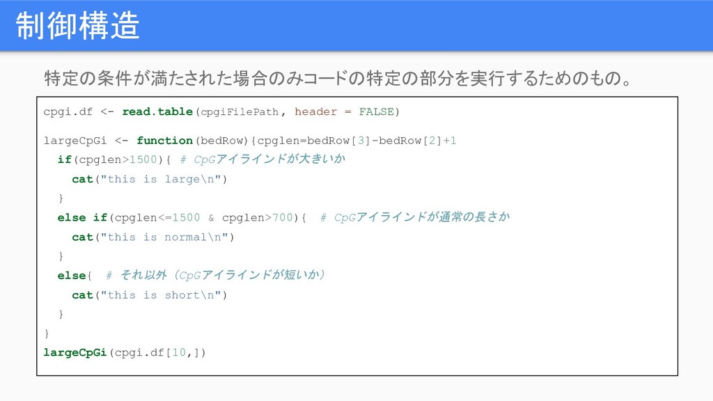
38. 制御構造 特定の条件が満たされた場合のみコードの特定の部分を実行するためのもの。 cpgi.df <- read.table(cpgiFilePath , header = FALSE) largeCpGi <- function(bedRow){cpglen=bedRow[3]-bedRow[2]+1 if(cpglen>1500){ # CpGアイラインドが大きいか cat("this is large\n") } else if(cpglen<=1500 & cpglen>700){　# CpGアイラインドが通常の長さか cat("this is normal\n") } else{　# それ以外（CpGアイラインドが短いか） cat("this is short\n") } } largeCpGi(cpgi.df[10,])
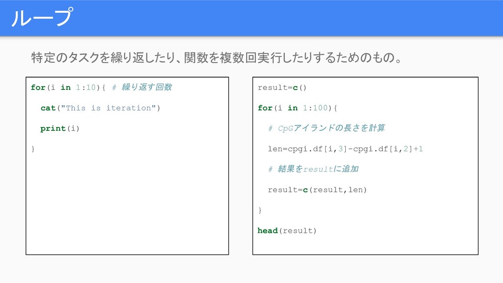
39. ループ 特定のタスクを繰り返したり、関数を複数回実行したりするためのもの。 for(i in 1:10){ # 繰り返す回数 cat("This is iteration") print(i) } result=c() for(i in 1:100){ # CpGアイランドの長さを計算 len=cpgi.df[i,3]-cpgi.df[i,2]+1 # 結果をresultに追加 result=c(result,len) } head(result)
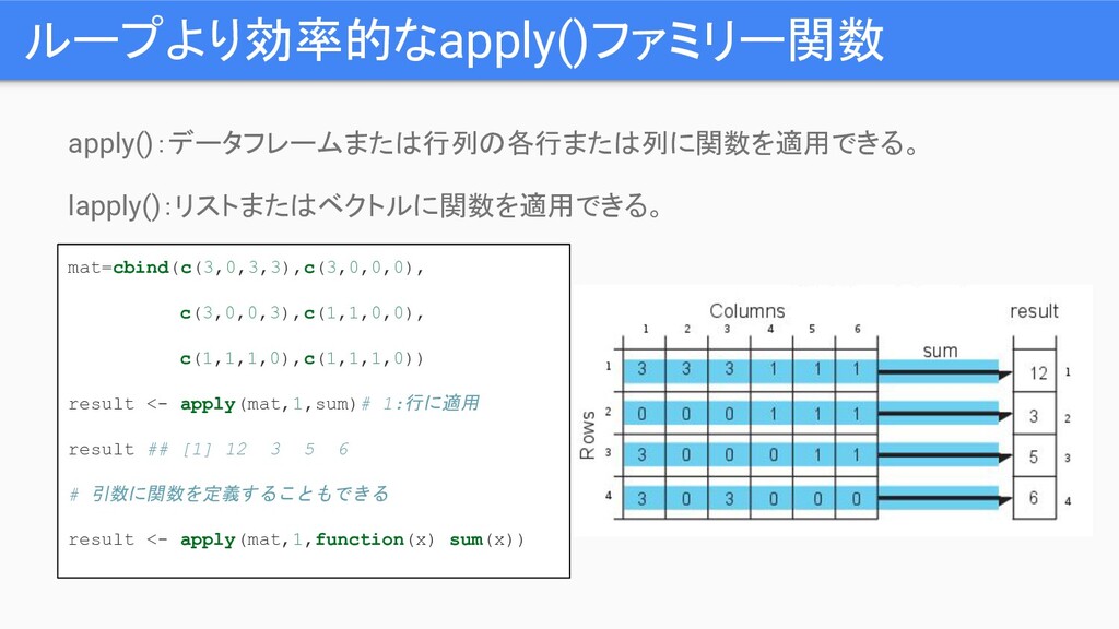
40. ループより効率的なapply()ファミリー関数 apply()：データフレームまたは行列の各行または列に関数を適用できる。 lapply()：リストまたはベクトルに関数を適用できる。 mat=cbind(c(3,0,3,3),c(3,0,0,0), c(3,0,0,3),c(1,1,0,0), c(1,1,1,0),c(1,1,1,0)) result <- apply(mat,1,sum)# 1:行に適用 result ## [1] 12 3 5 6 # 引数に関数を定義することもできる result <- apply(mat,1,function(x) sum(x))
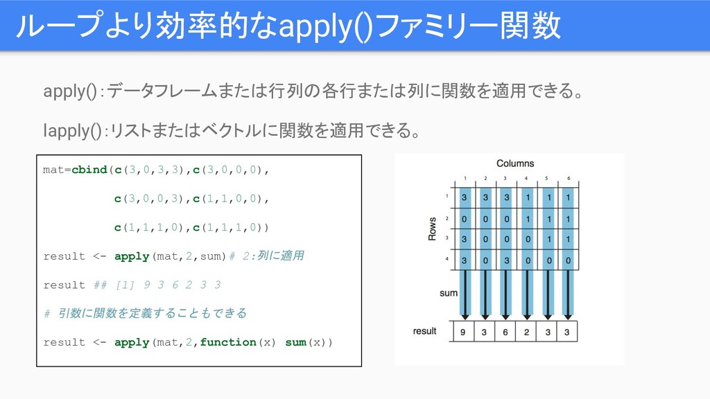
41. ループより効率的なapply()ファミリー関数 apply()：データフレームまたは行列の各行または列に関数を適用できる。 lapply()：リストまたはベクトルに関数を適用できる。 mat=cbind(c(3,0,3,3),c(3,0,0,0), c(3,0,0,3),c(1,1,0,0), c(1,1,1,0),c(1,1,1,0)) result <- apply(mat,2,sum)# 2:列に適用 result ## [1] 9 3 6 2 3 3 # 引数に関数を定義することもできる result <- apply(mat,2,function(x) sum(x))
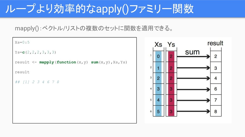
42. ループより効率的なapply()ファミリー関数 mapply()：ベクトル/リストの複数のセットに関数を適用できる。 Xs=0:5 Ys=c(2,2,2,3,3,3) result <- mapply(function(x,y) sum(x,y),Xs,Ys) result ## [1] 2 3 4 6 7 8
43. ベクトル化された関数 汎用性が高い一部の関数で内部的に組み込まれた関数 ※ベクトル化された関数は一部なので、遅かれ早かれapply()ファミリーの適用が必要になる。 result=Xs+Ys　# mapply()とsum()を適用しなくても、すでにベクトル化された“+”を使用できる。 result ## [1] 2 3 4 6 7 8 colSums(mat) # 列の和 ## [1] 9 3 6 2 3 3 rowSums(mat) # 行の和 ## [1] 12 3 5 6
44. 参考：Rオンライン学習サイト DataCamp: Learn R, Python & Data Science Online Dataquest: Learn R, Python and SQL for Data Science