Statistical Rethinking 2022 Lecture 06

Course materials: https://github.com/rmcelreath/stat_rethinking_2022

Transcript

1. Statistical Rethinking 06: Good & Bad Controls 2022
2. G P U C grandparent education parent education child education unobserved confound
3. G P C P is a mediator
4. G P U C P is a collider
5. G P U C Can estimate total effect of G on C Cannot estimate direct effect G P U C C i ∼ Normal(μ i , σ) μ i = α + β G G i C i ∼ Normal(μ i , σ) μ i = α + β G G i + β P P i
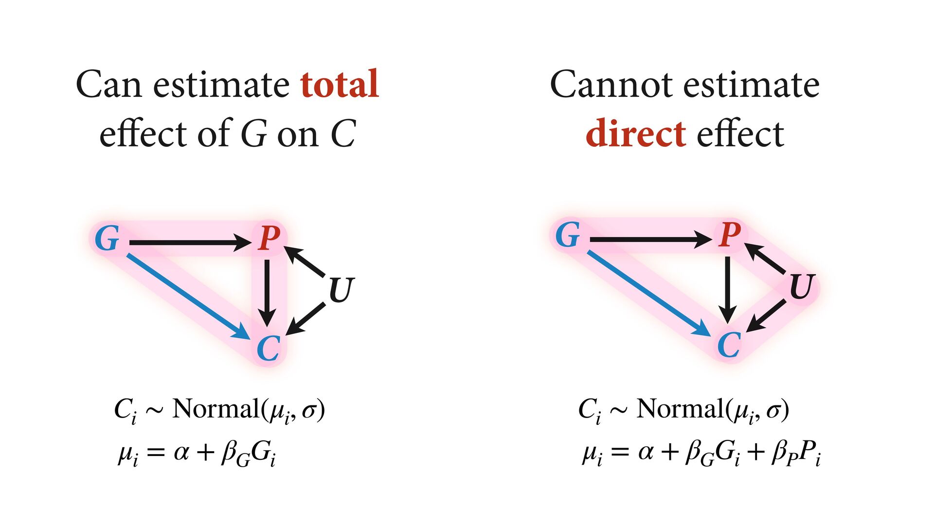
6. N <- 200 # num grandparent-parent-child triads b_GP <- 1 # direct effect of G on P b_GC <- 0 # direct effect of G on C b_PC <- 1 # direct effect of P on C b_U <- 2 #direct effect of U on P and C set.seed(1) U <- 2*rbern( N , 0.5 ) - 1 G <- rnorm( N ) P <- rnorm( N , b_GP*G + b_U*U ) C <- rnorm( N , b_PC*P + b_GC*G + b_U*U ) d <- data.frame( C=C , P=P , G=G , U=U ) m6.11 <- quap( alist( C ~ dnorm( mu , sigma ), mu <- a + b_PC*P + b_GC*G, a ~ dnorm( 0 , 1 ), c(b_PC,b_GC) ~ dnorm( 0 , 1 ), sigma ~ dexp( 1 ) ), data=d ) Page 180 b_GC b_PC -1.0 -0.5 0.0 0.5 1.0 1.5 Value True values
7. Stratify by parent centile (collider) Two ways for parents to attain their education: from G or from U b_GC b_PC -1.0 -0.5 0.0 0.5 1.0 1.5 Value
8. From Theory to Estimate Our job is to (1) Clearly state assumptions (2) Deduce implications (3) Test implications
9. Avoid Being Clever At All Costs Being clever is neither reliable nor transparent Now what? Given a causal model, can use logic to derive implications Others can use same logic to verify/ challenge your work
10. X Z Y The Pipe X Z Y The Fork X Z Y The Collider X and Y associated unless stratify by Z X and Y associated unless stratify by Z X and Y not associated unless stratify by Z
11. A B C X Z Y F G
12. A B C X Z Y F G Forks
13. A B C X Z Y F G Forks Pipes
14. A B C X Z Y F G Forks Pipes Colliders
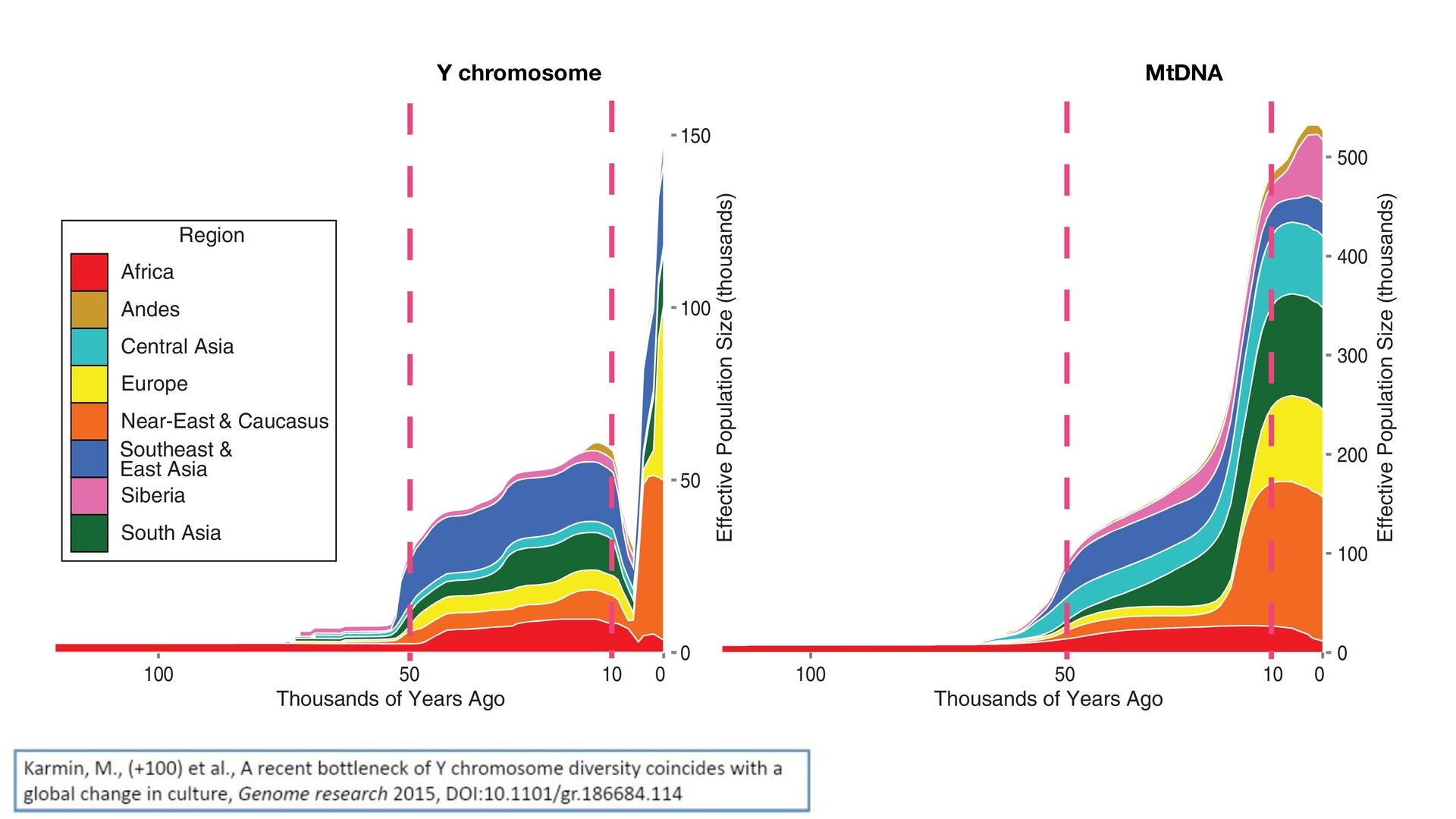
15. Thousands of Years Ago 0 50 100 150 0 50 100 Effective Population Size (thousands) Effective Population Size (thousands) Thousands of Years Ago 0 100 200 300 400 500 0 50 100 Africa Andes Central Asia Europe Near-East & Caucasus Southeast & East Asia Siberia South Asia Region 10 10 2. Cumulative Bayesian skyline plots of Y chromosome and mtDNA diversity by world regions. The red dashed lines highlight the horizons d 50 kya. Individual plots for each region are presented in Supplemental Figure S4A. Y chromosome MtDNA
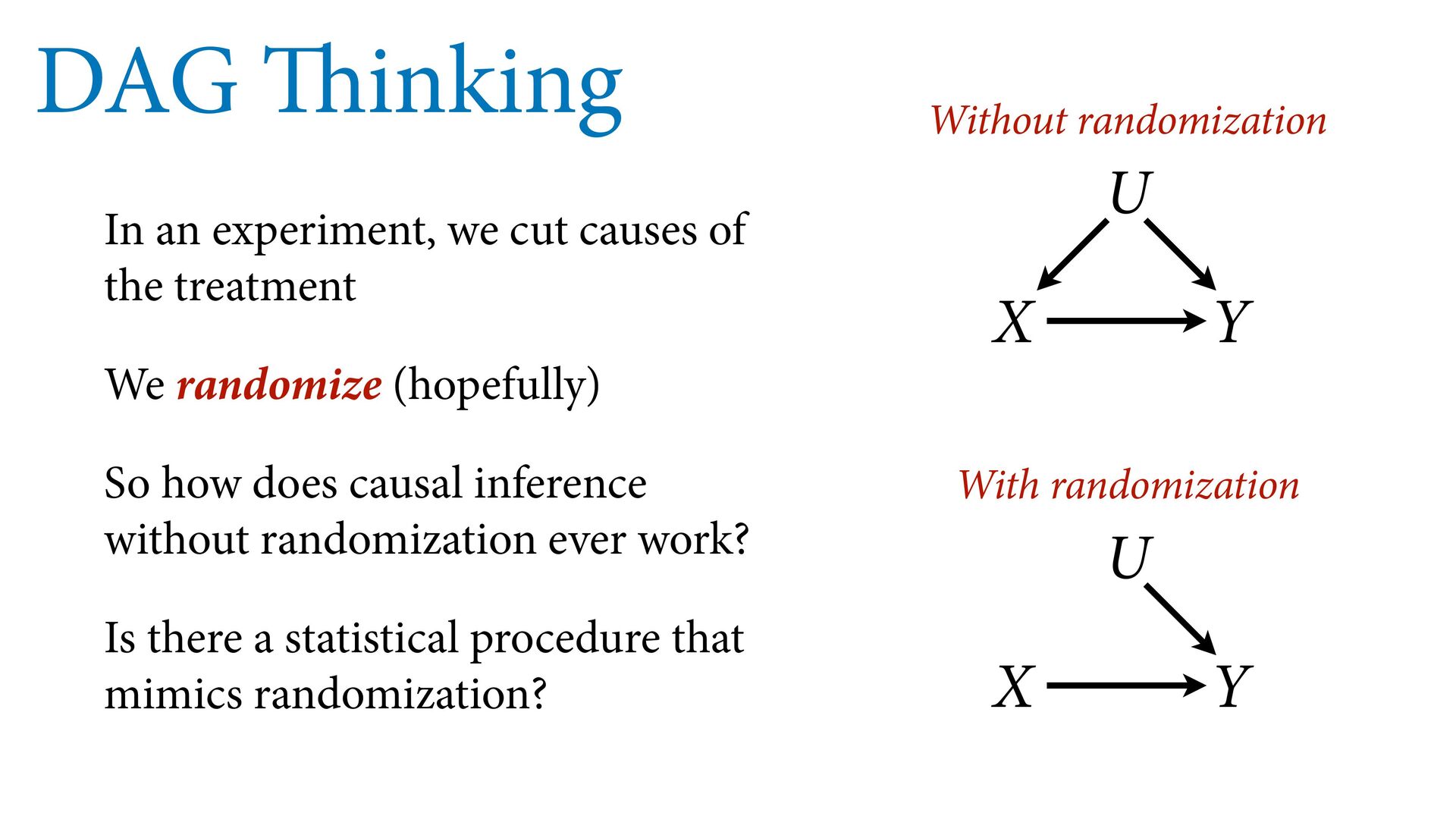
16. DAG Thinking In an experiment, we cut causes of the treatment We randomize (hopefully) So how does causal inference without randomization ever work? Is there a statistical procedure that mimics randomization? X Y U Without randomization X Y U With randomization
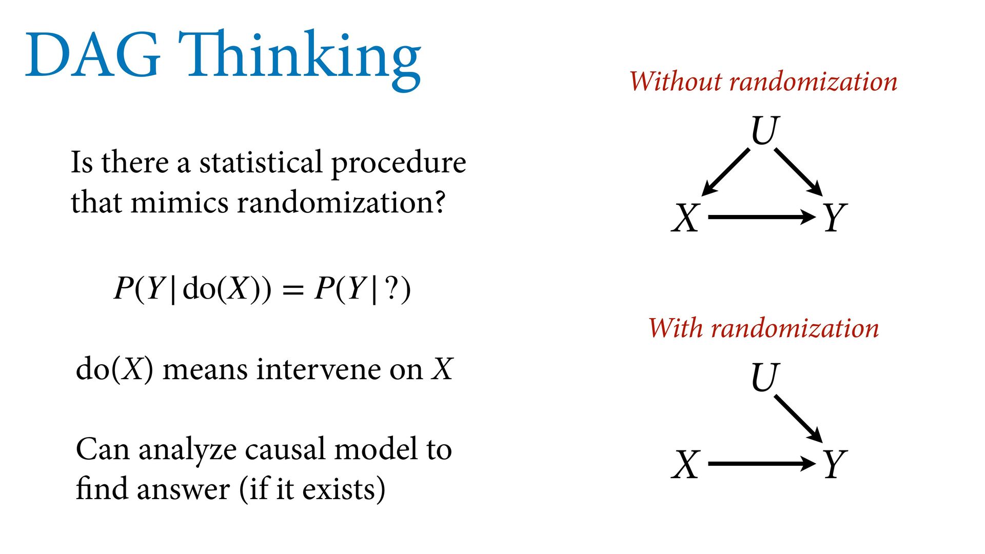
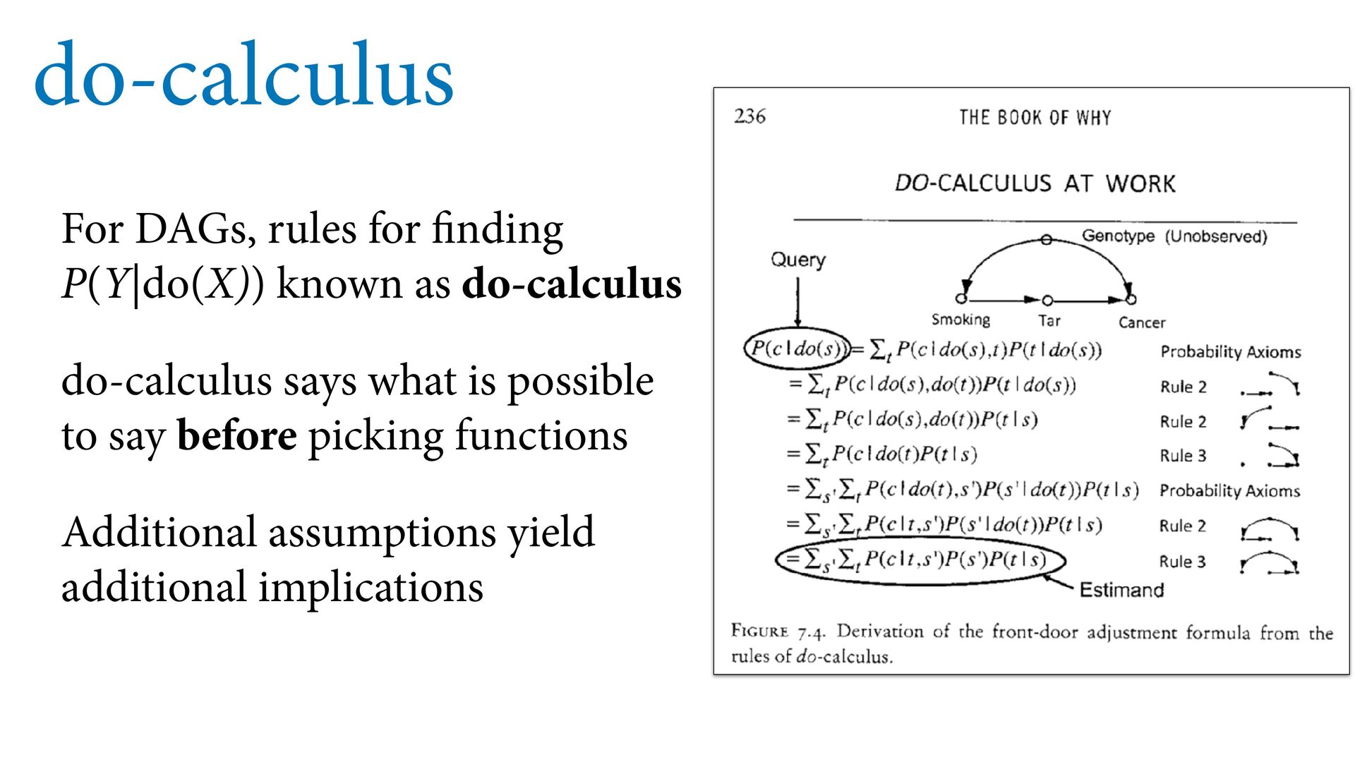
17. DAG Thinking Is there a statistical procedure that mimics randomization? X Y U Without randomization X Y U With randomization P(Y|do(X)) = P(Y|?) do(X) means intervene on X
 
 Can analyze causal model to find answer (if it exists)
18. Example: Simple Confound X Y U
19. Example: Simple Confound X Y U Non-causal path
 X <– U –> Y
 
 Close the fork!
 Condition on U
20. Example: Simple Confound X Y U Non-causal path
 X <– U –> Y
 
 Close the fork!
 Condition on U
21. Example: Simple Confound X Y U Non-causal path
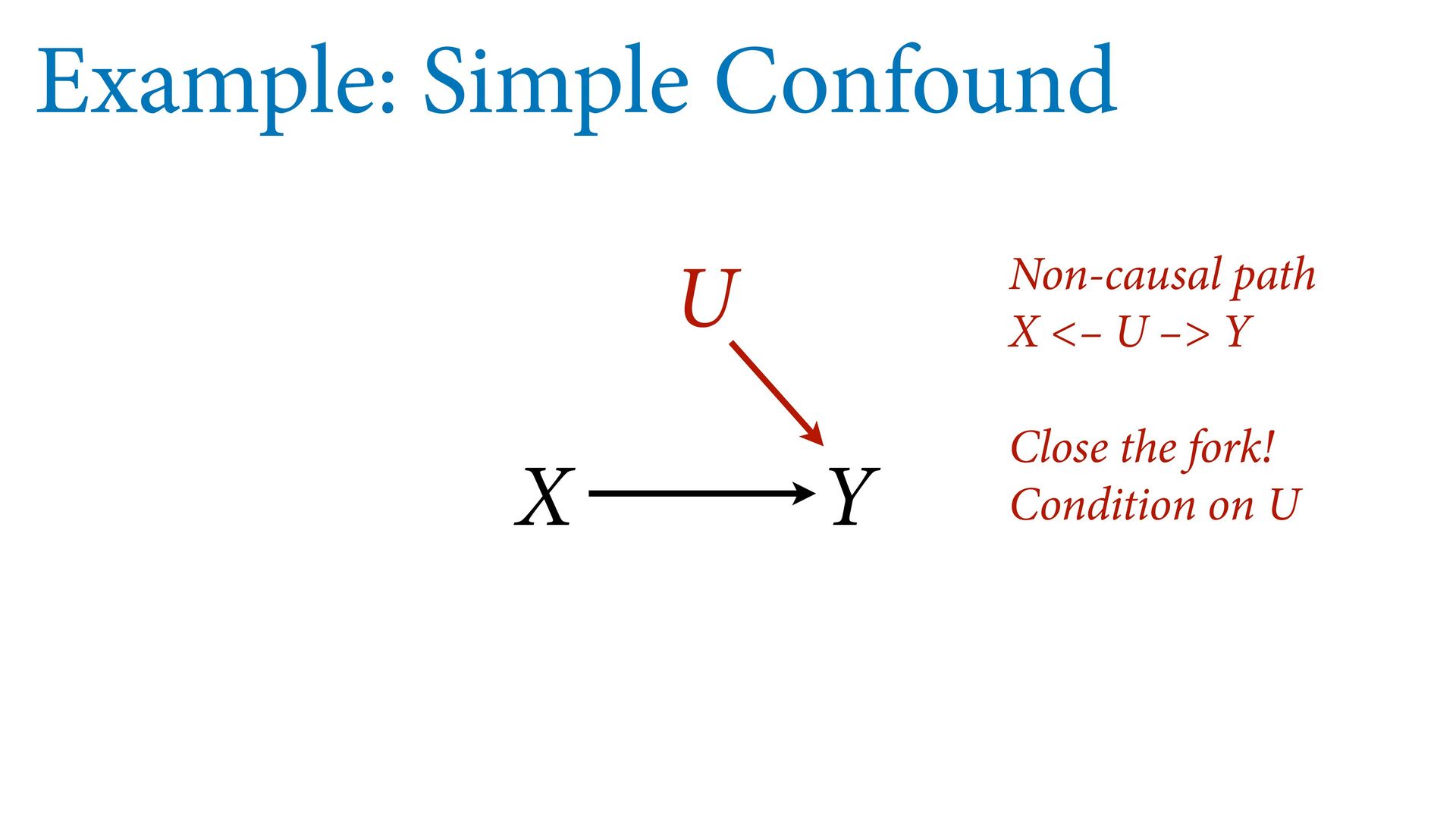
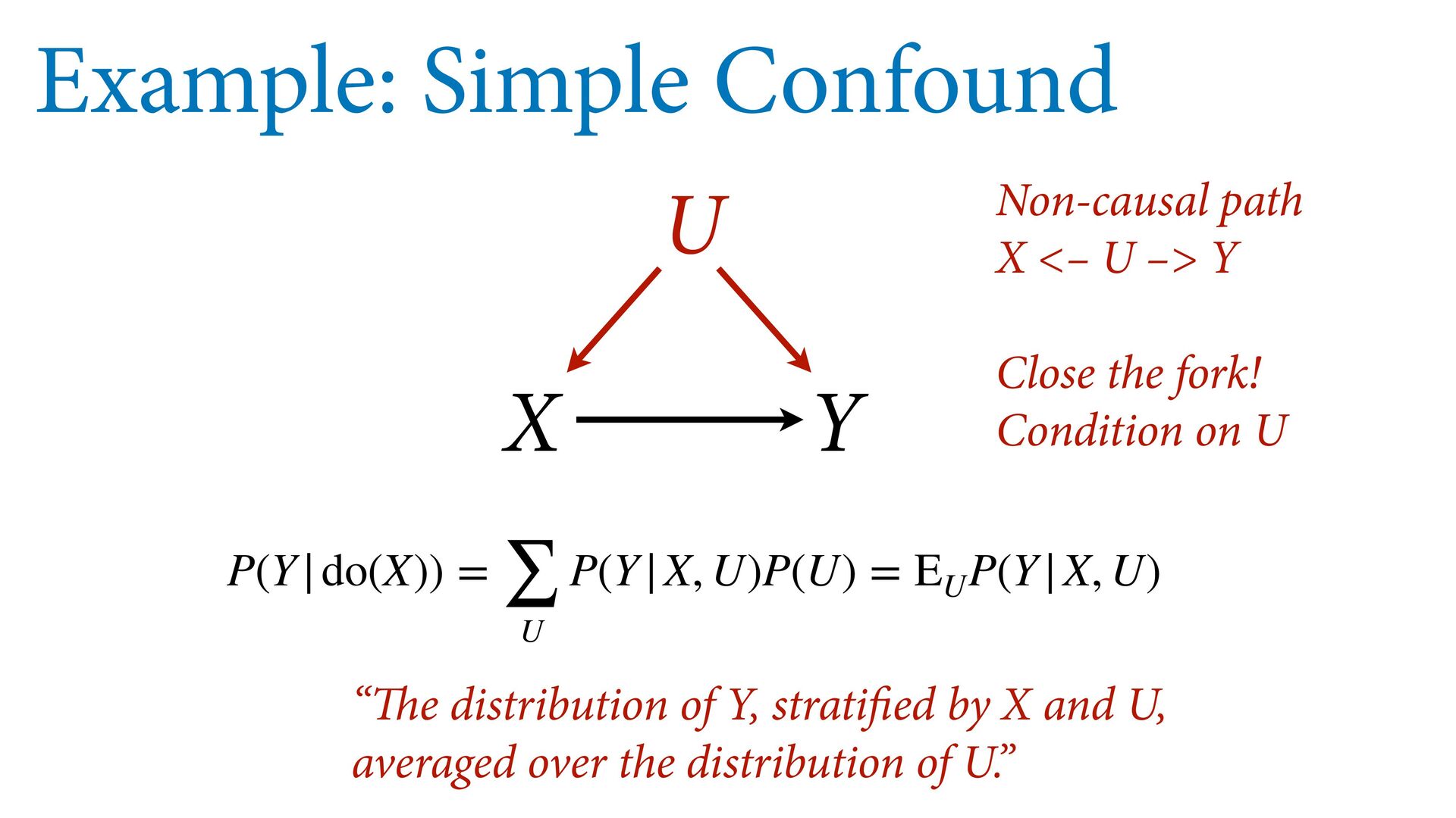
 X <– U –> Y
 
 Close the fork!
 Condition on U P(Y|do(X)) = ∑ U P(Y|X, U)P(U) = E U P(Y|X, U) “The distribution of Y, stratified by X and U, averaged over the distribution of U.”
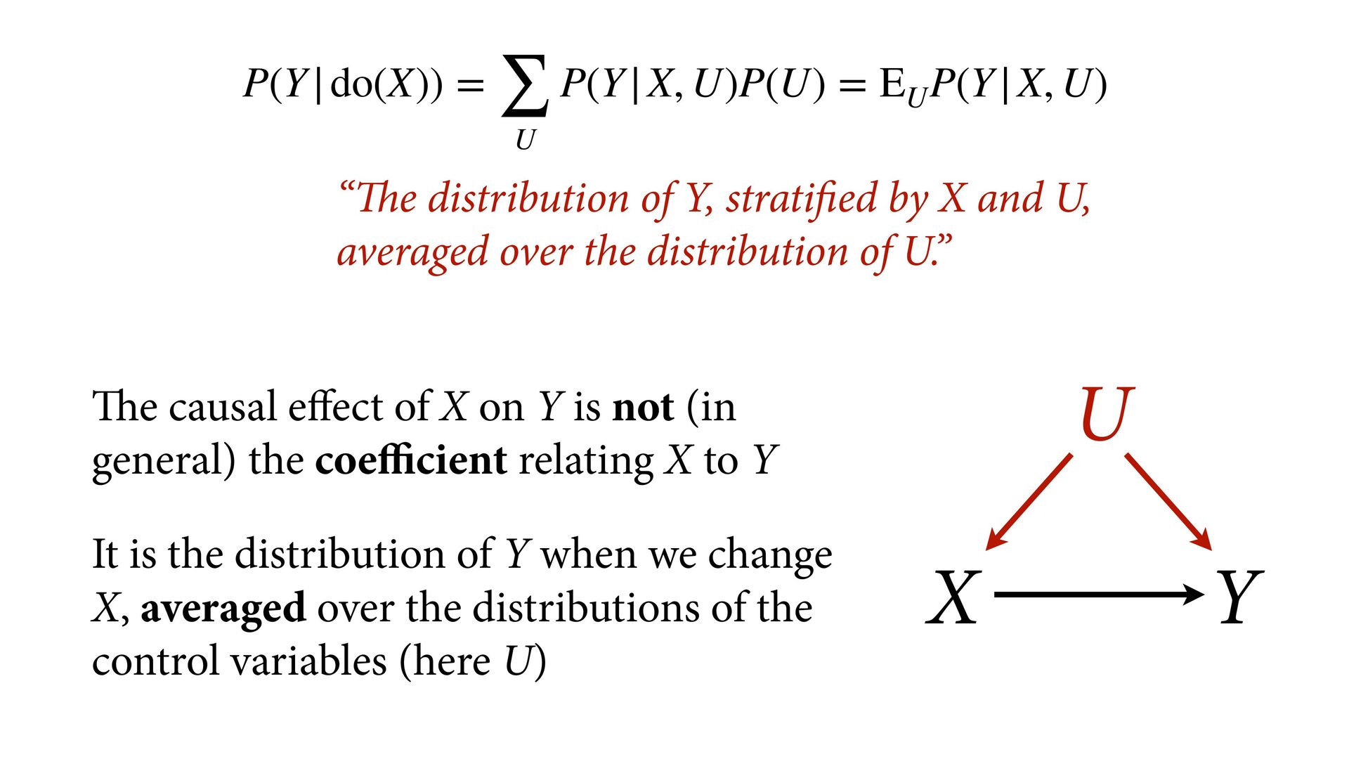
22. The causal effect of X on Y is not (in general) the coefficient relating X to Y It is the distribution of Y when we change X, averaged over the distributions of the control variables (here U) P(Y|do(X)) = ∑ U P(Y|X, U)P(U) = E U P(Y|X, U) “The distribution of Y, stratified by X and U, averaged over the distribution of U.” X Y U
23. Marginal Effects Example B G C cheetahs baboons gazelle
24. Marginal Effects Example B G C cheetahs present B G C cheetahs absent Causal effect of baboons depends upon distribution of cheetahs
25. do-calculus For DAGs, rules for finding 
 P(Y|do(X)) known as do-calculus do-calculus says what is possible to say before picking functions Additional assumptions yield additional implications
26. do-calculus do-calculus is worst case: additional assumptions often allow stronger inference do-calculus is best case: 
 if inference possible by do- calculus, does not depend on special assumptions Judea Pearl, father of do-calculus, in 1966
27. Backdoor Criterion Very useful implication of do-calculus is the Backdoor Criterion Backdoor Criterion is a shortcut to applying rules of do-calculus Also inspires strategies for research design that yield valid estimates
28. Backdoor Criterion Backdoor Criterion: Rule to find a set of variables to stratify (condition) by to yield P(Y|do(X))
29. Backdoor Criterion Backdoor Criterion: Rule to find a set of variables to stratify (condition) by to yield P(Y|do(X)) (1) Identify all paths connection the treatment (X) to the outcome (Y)
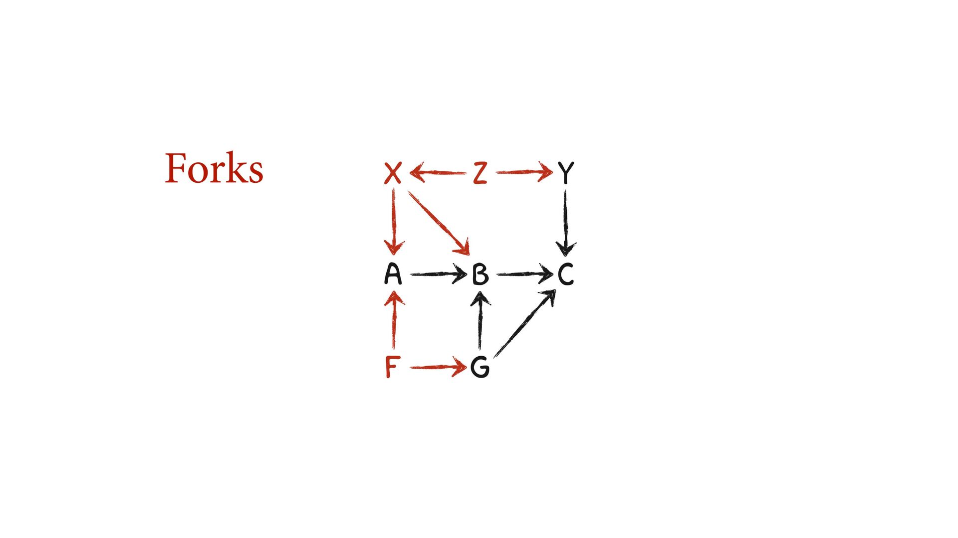
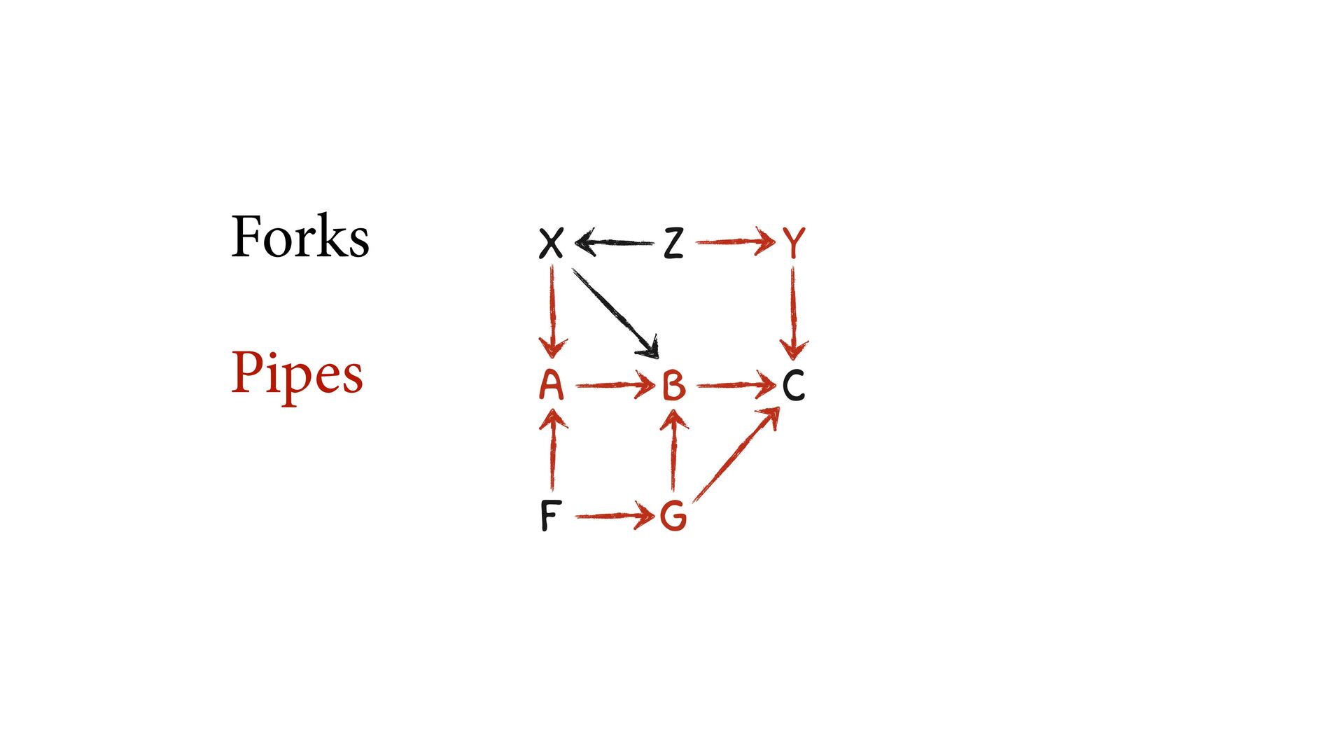
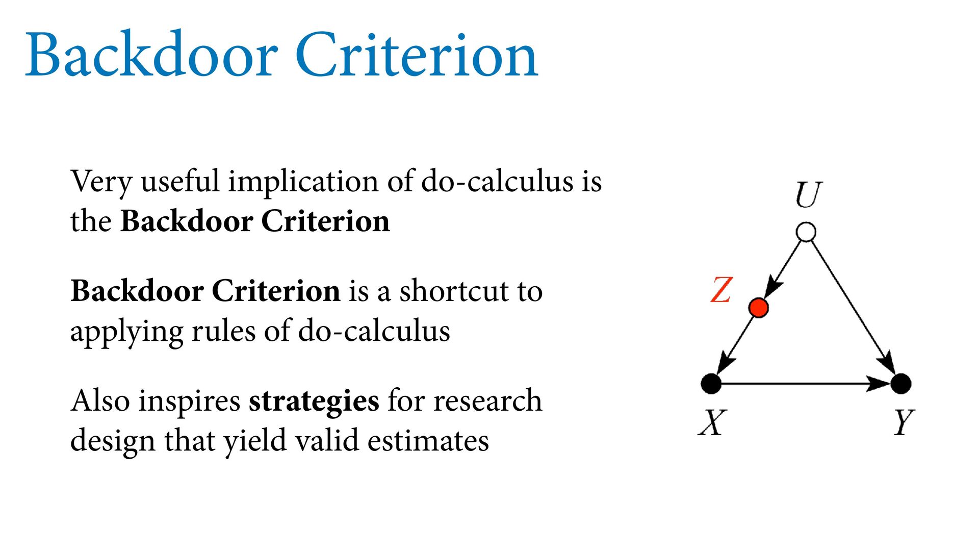
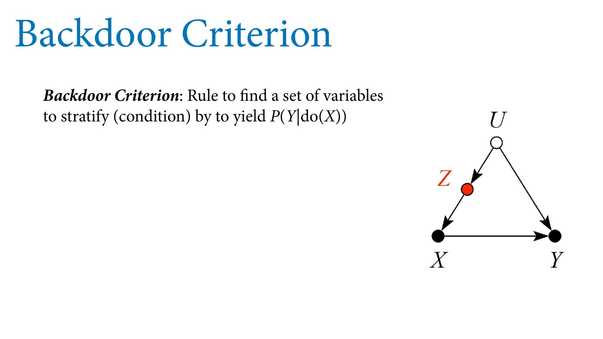
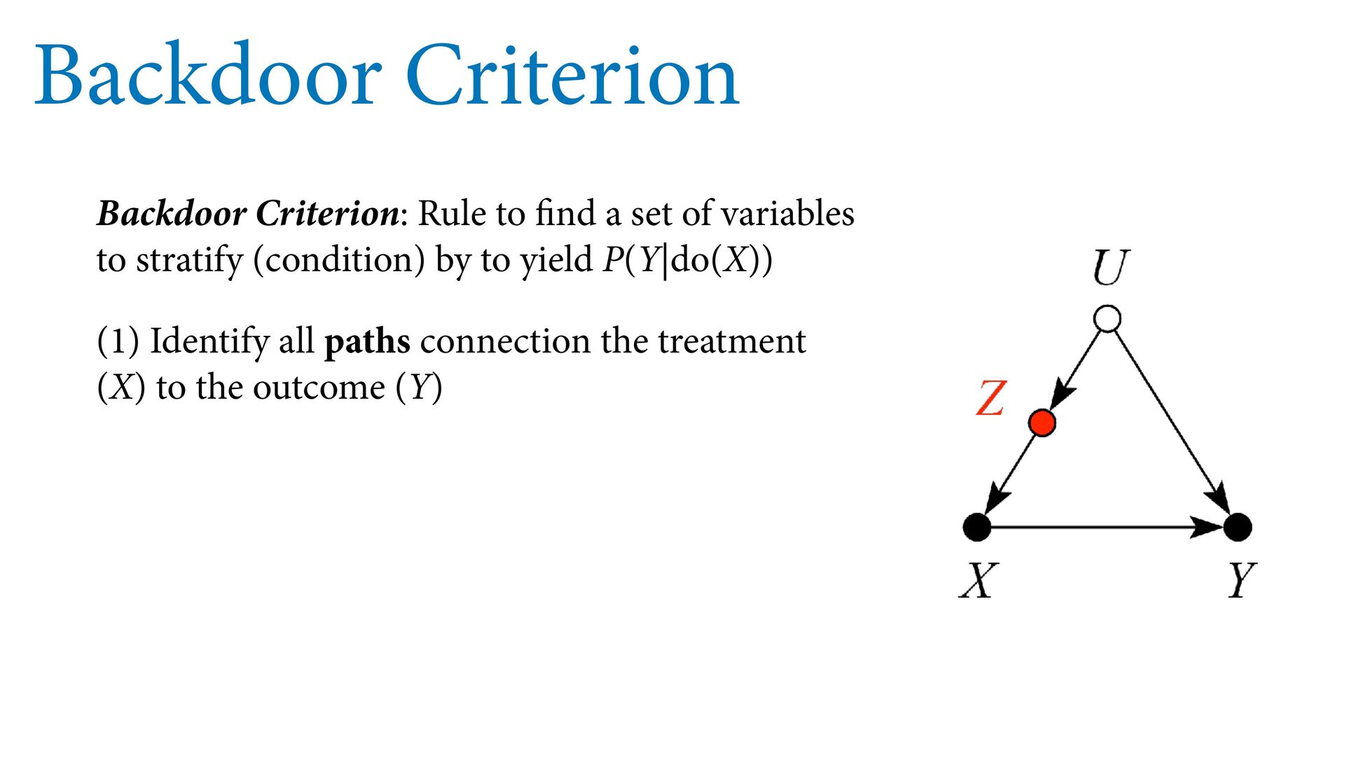
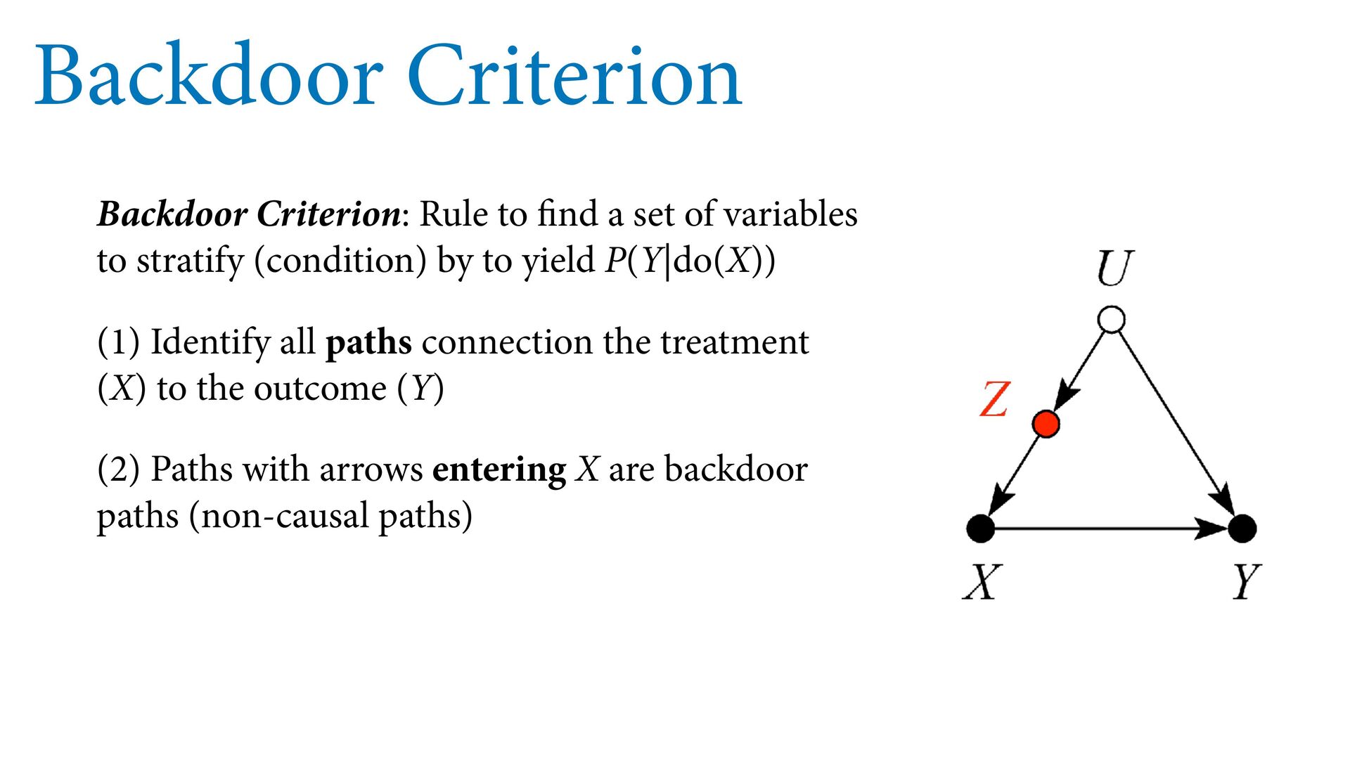
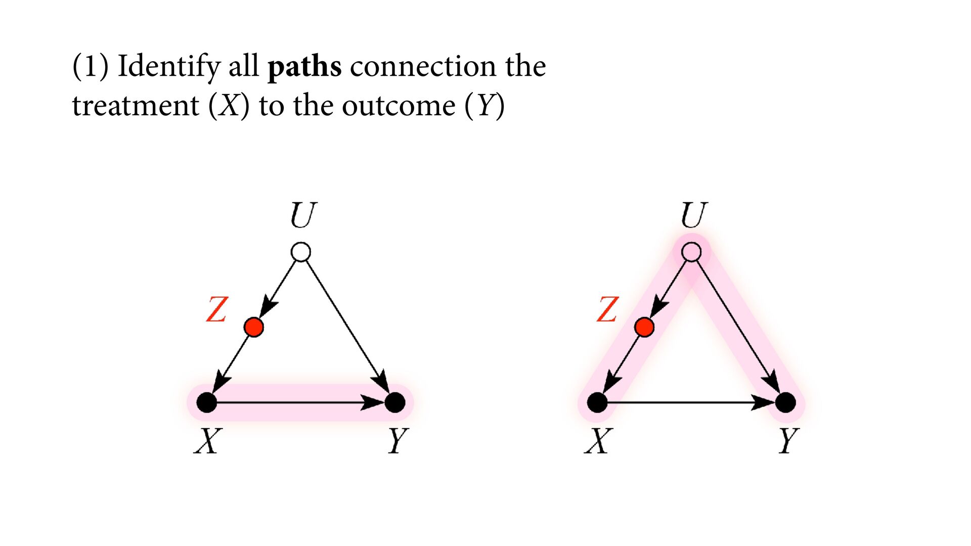
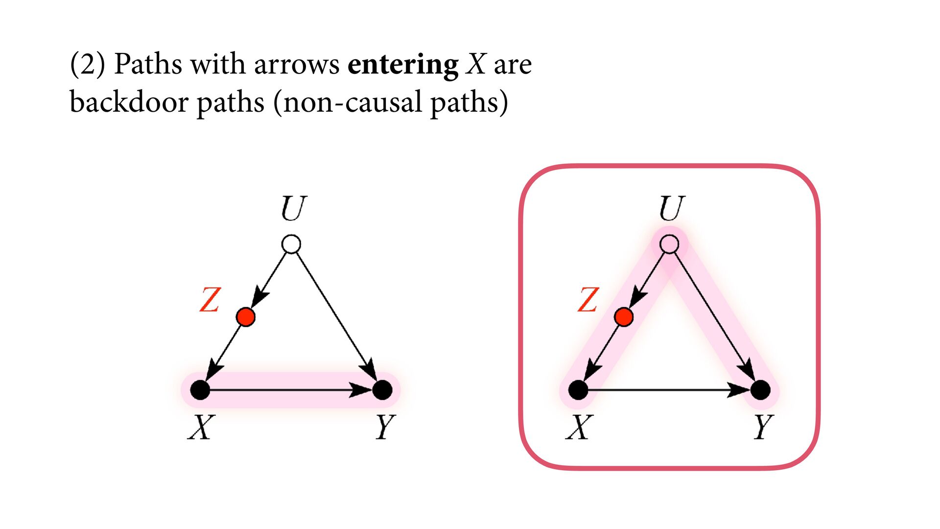
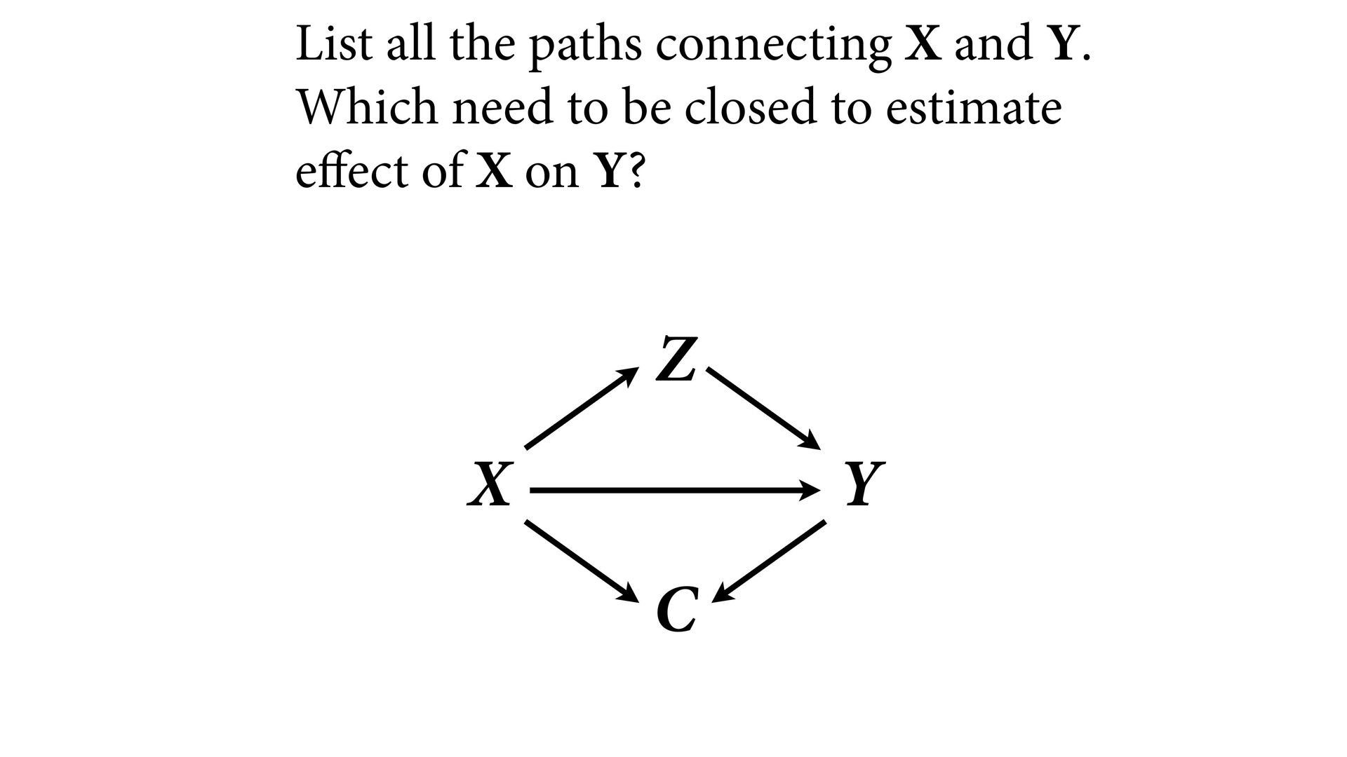
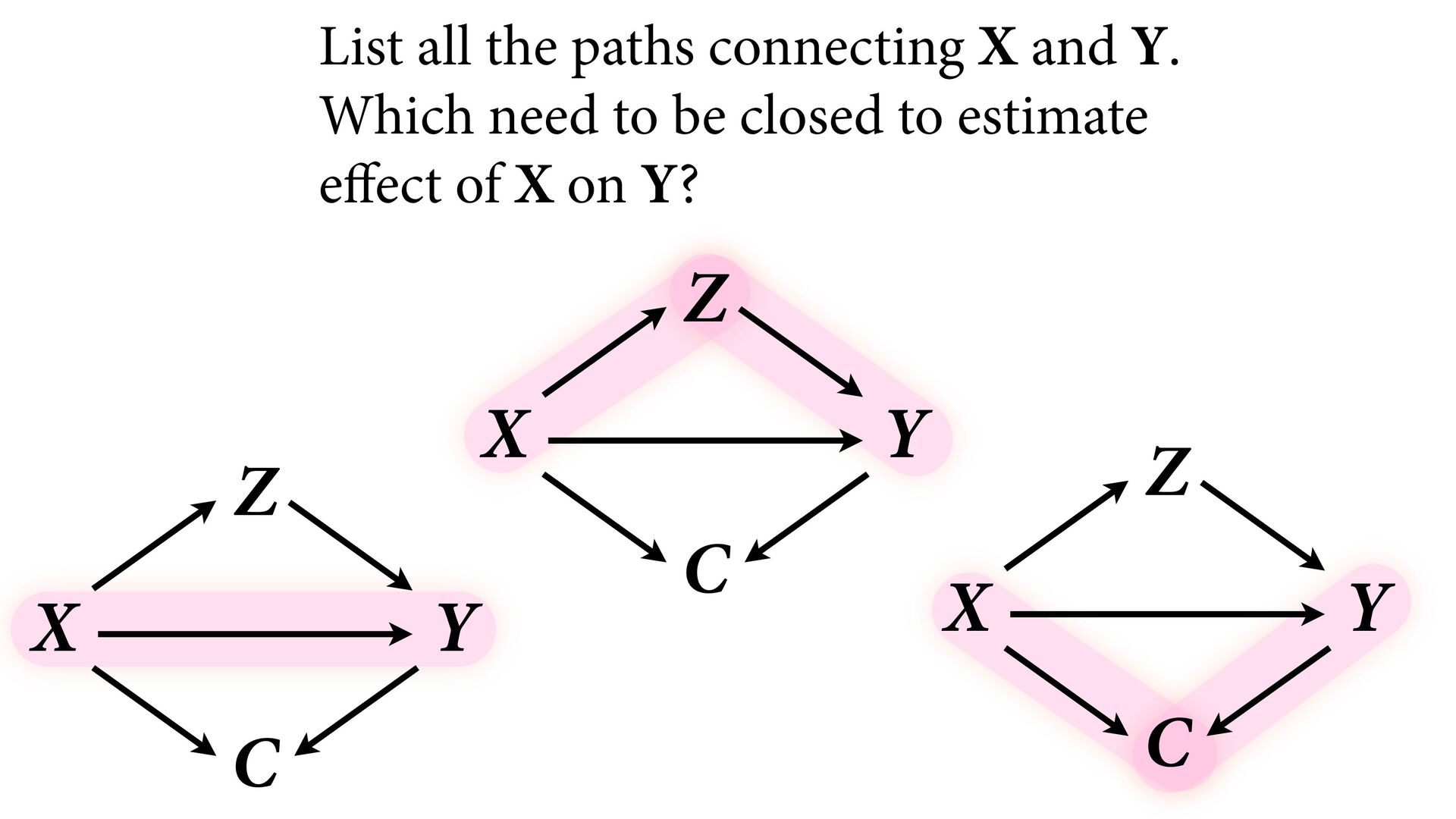
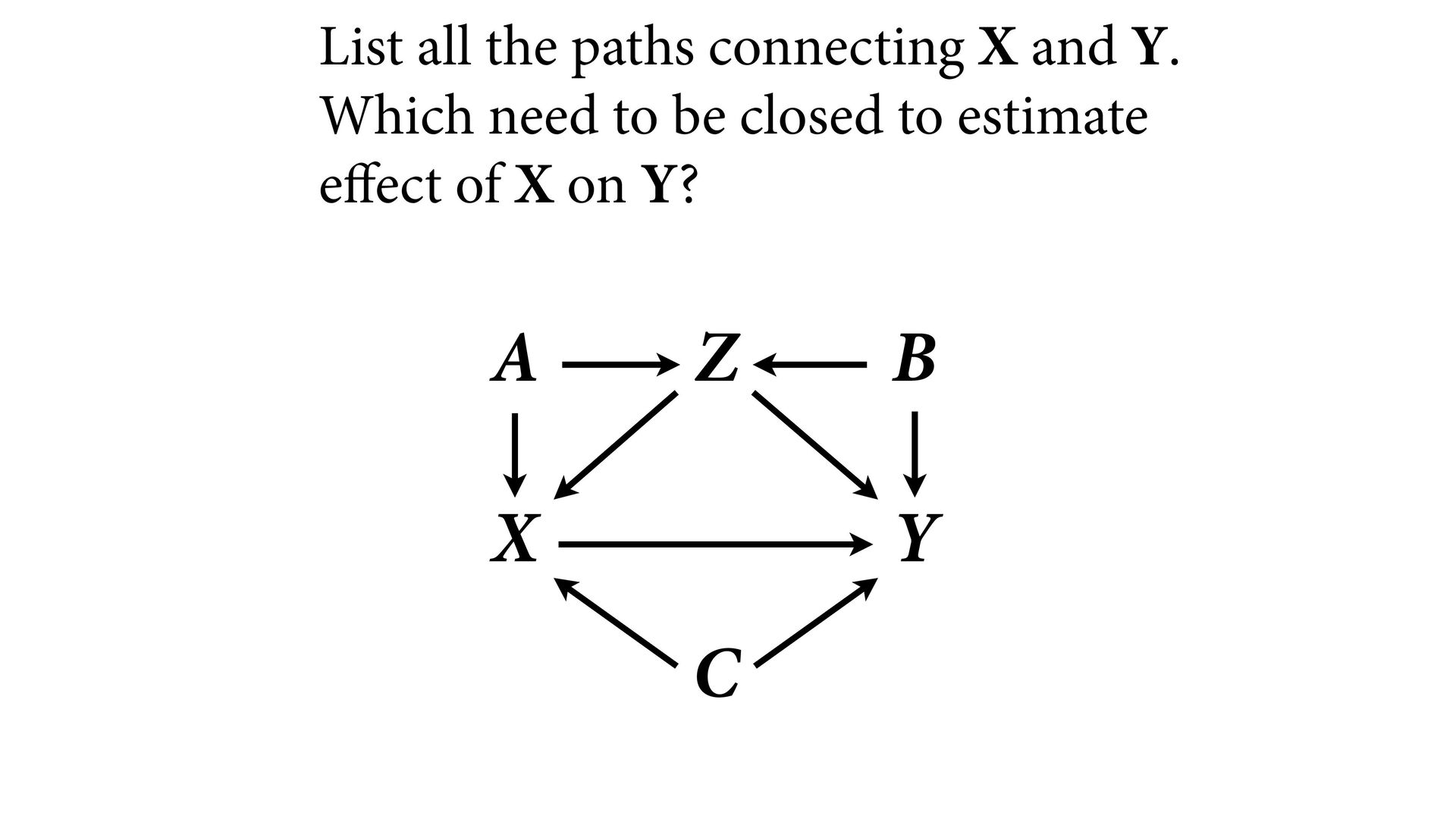
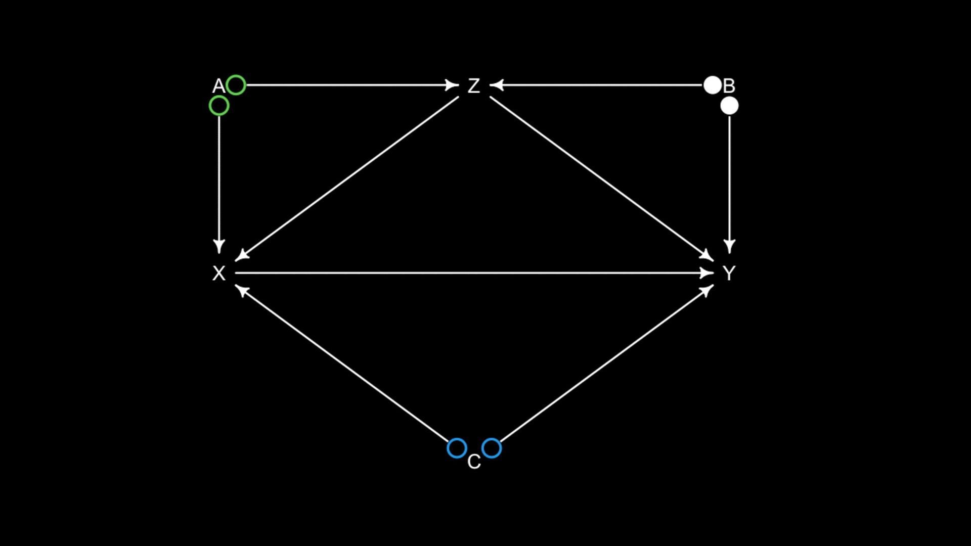
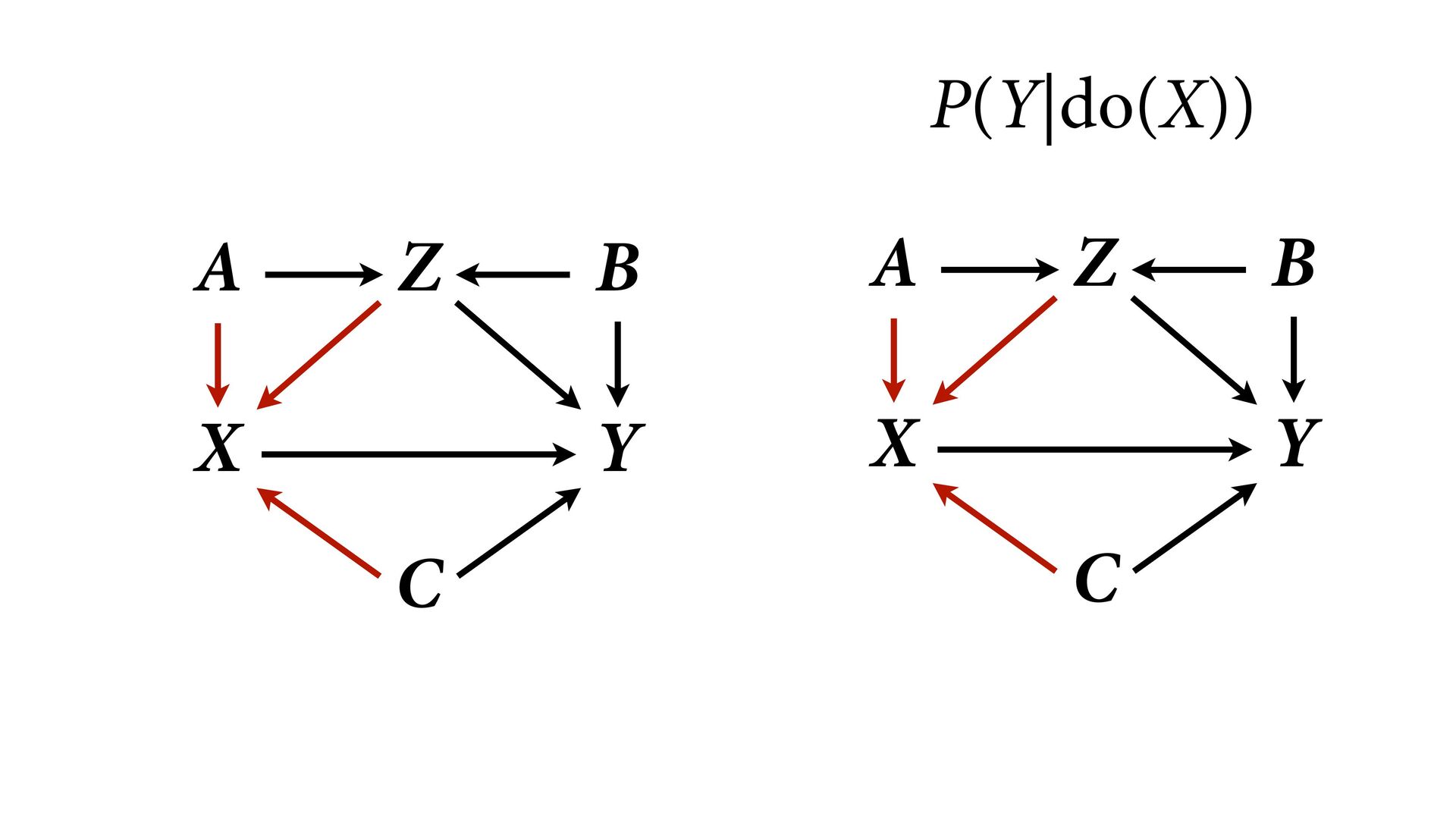
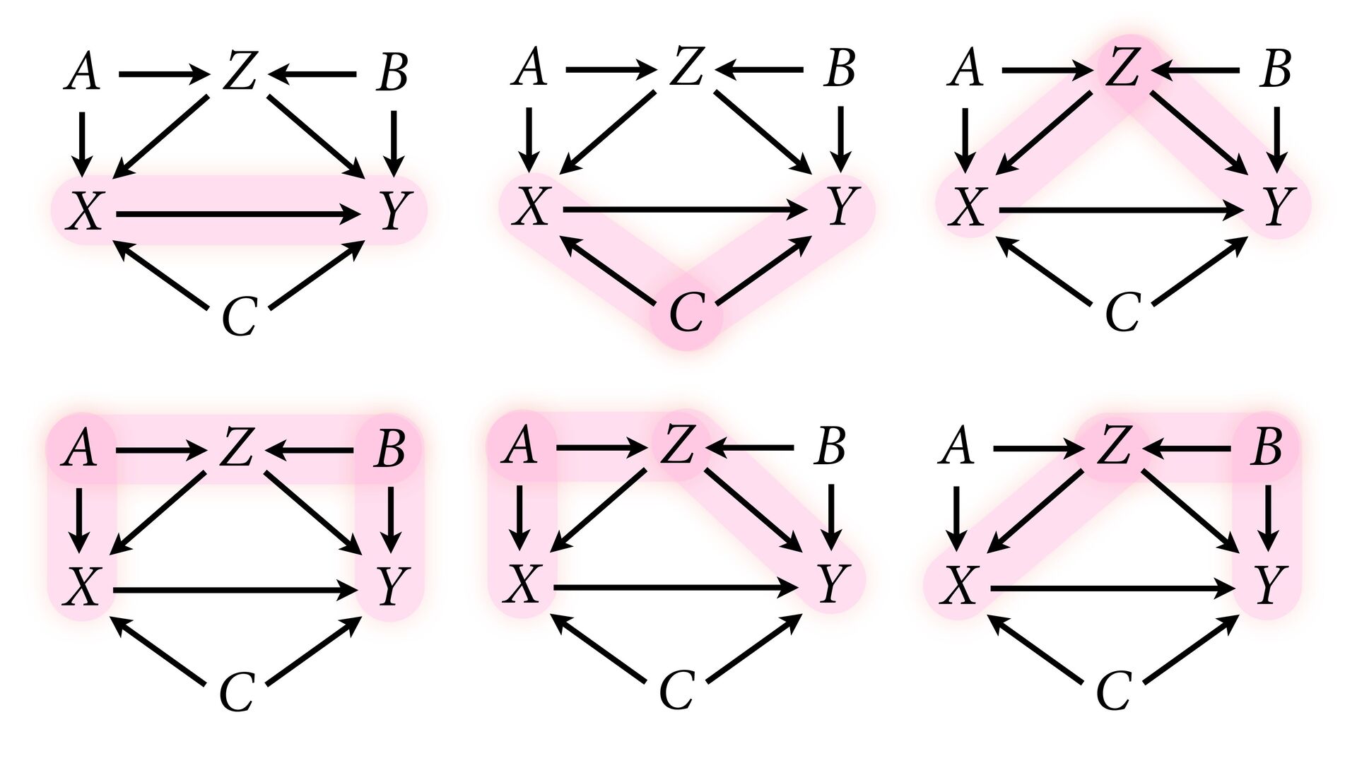
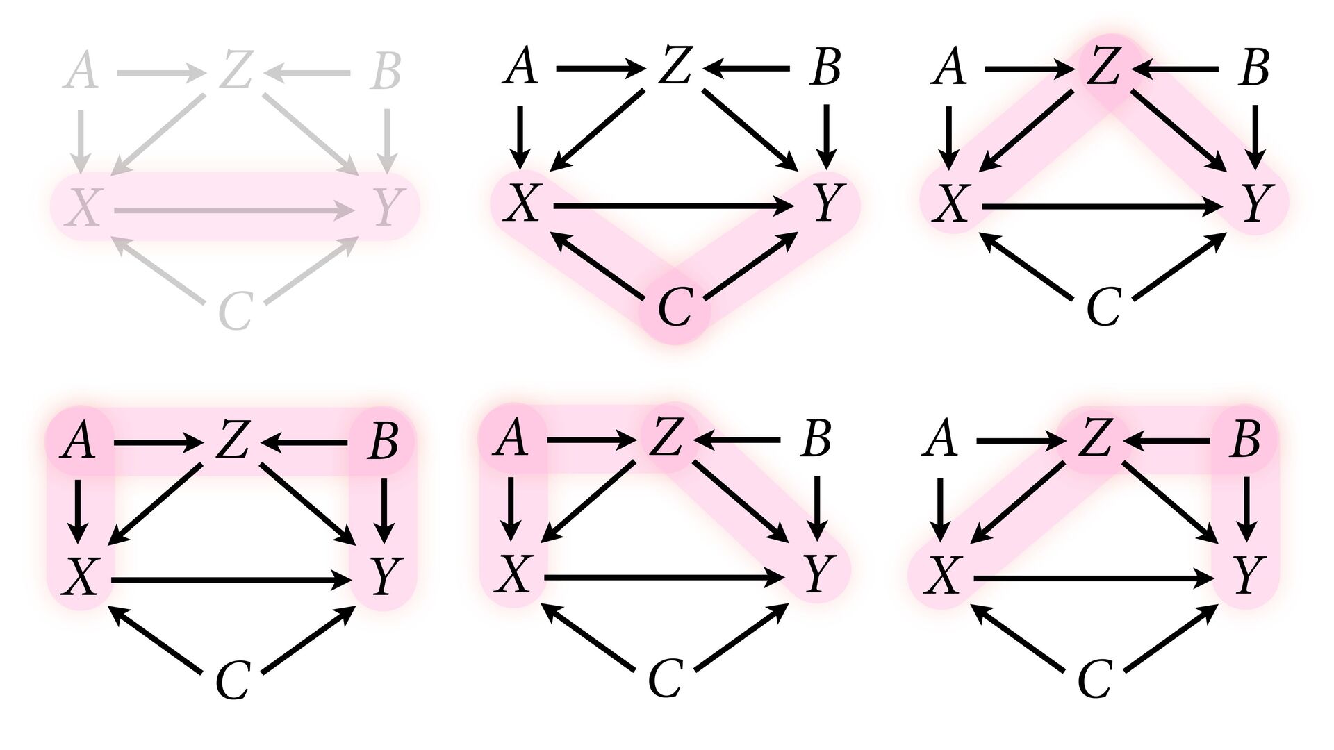
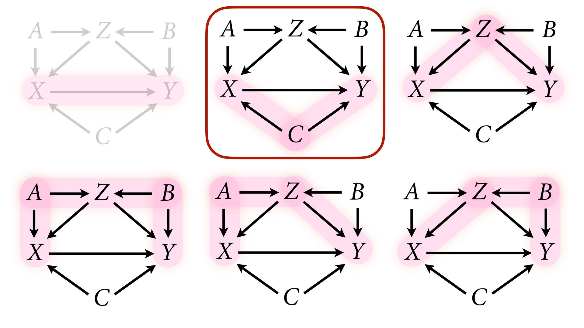
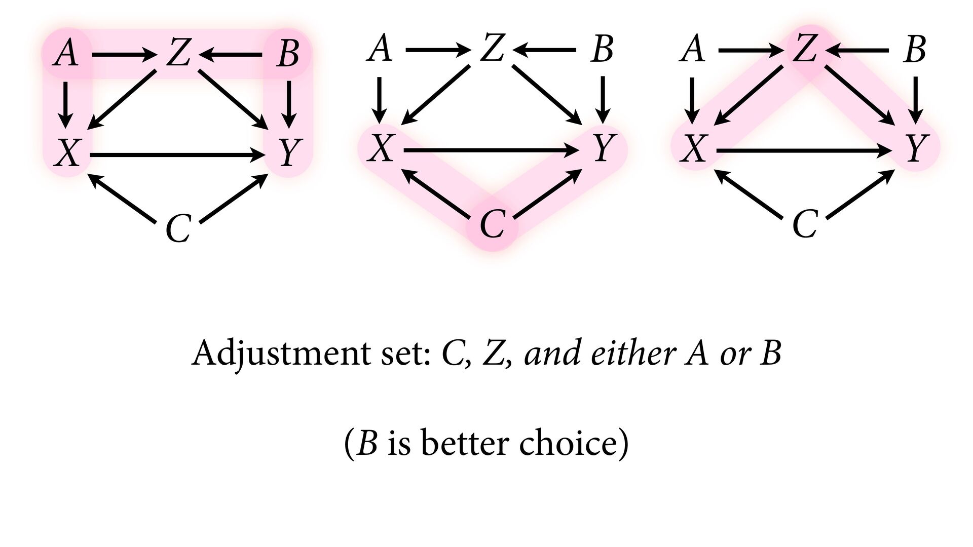
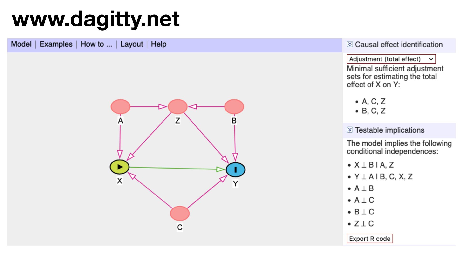
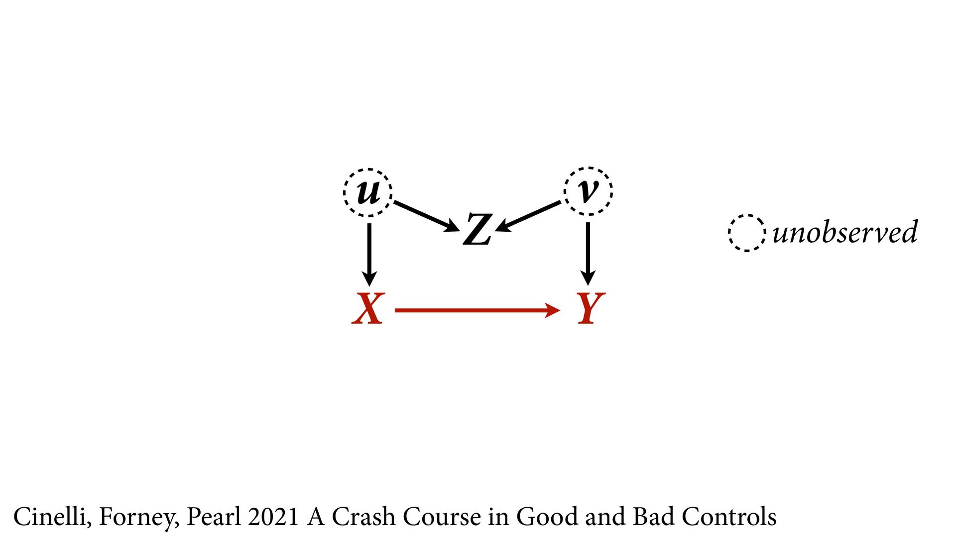
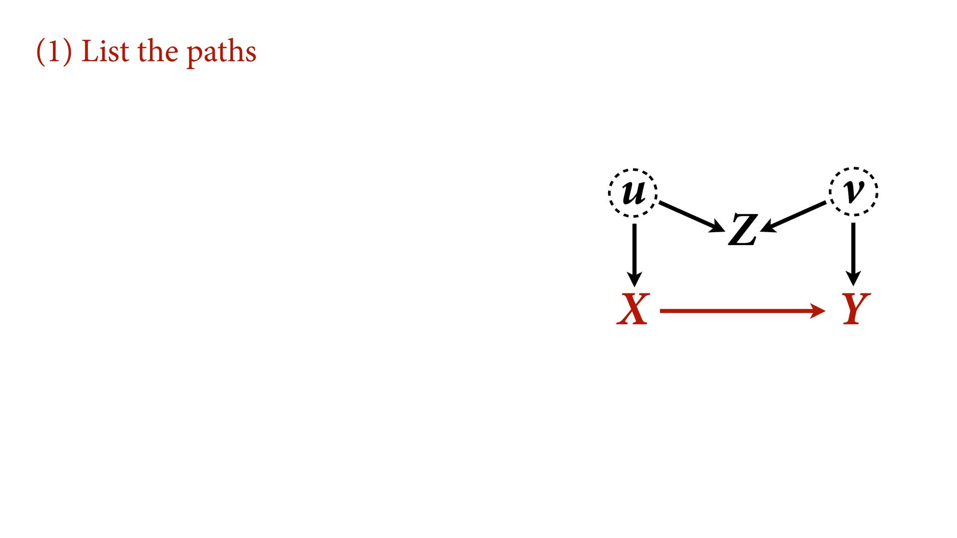
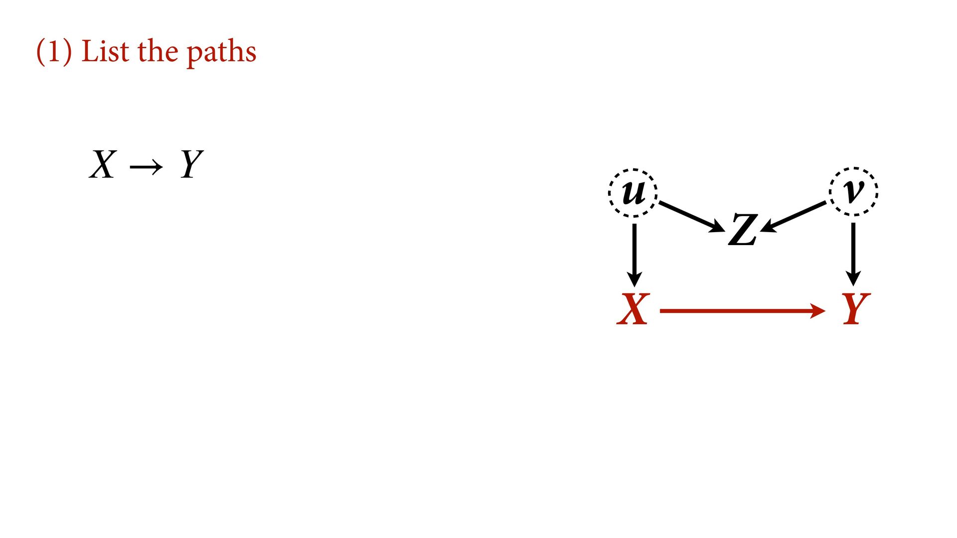
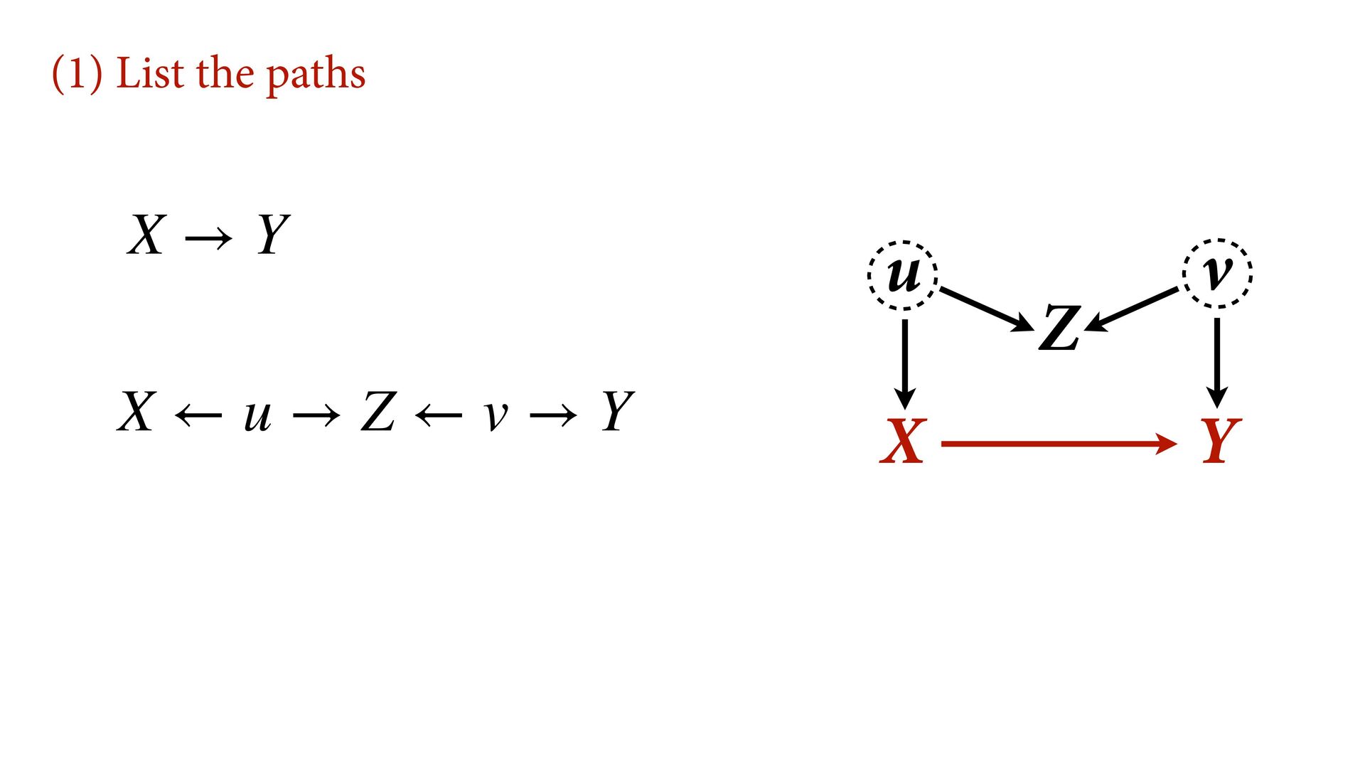
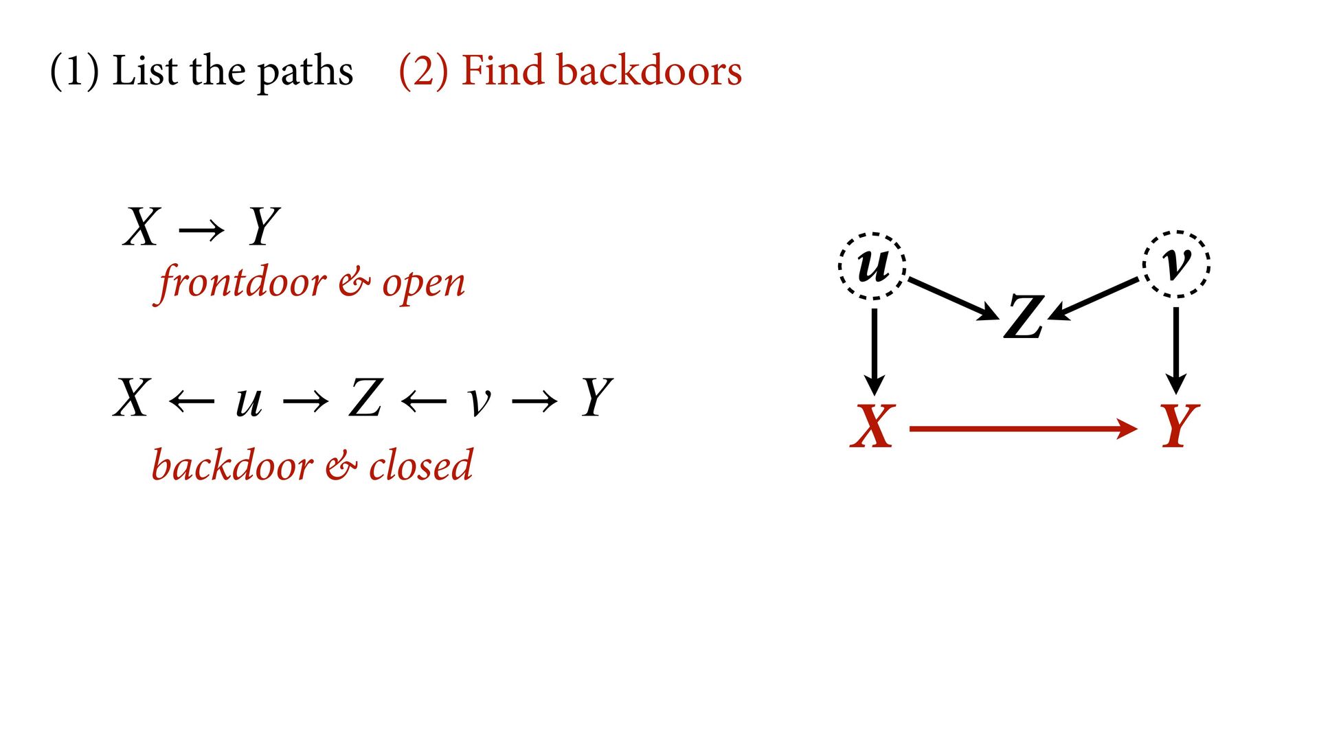
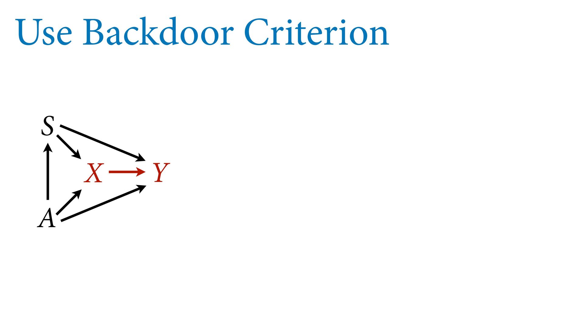
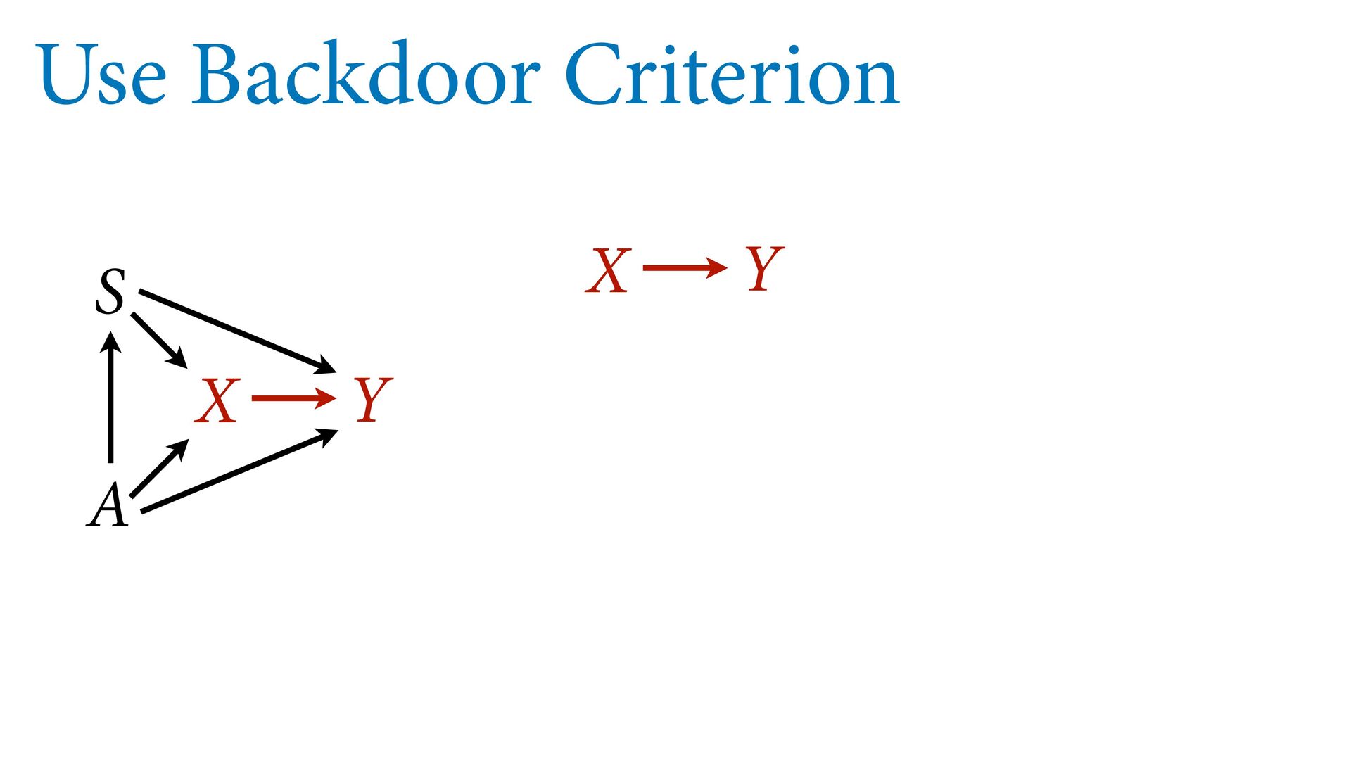
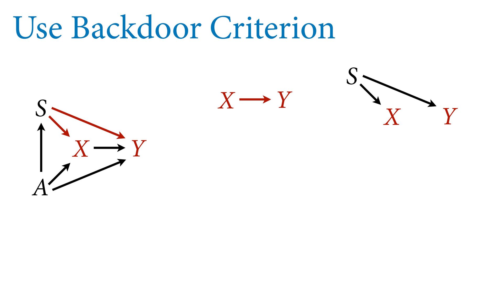
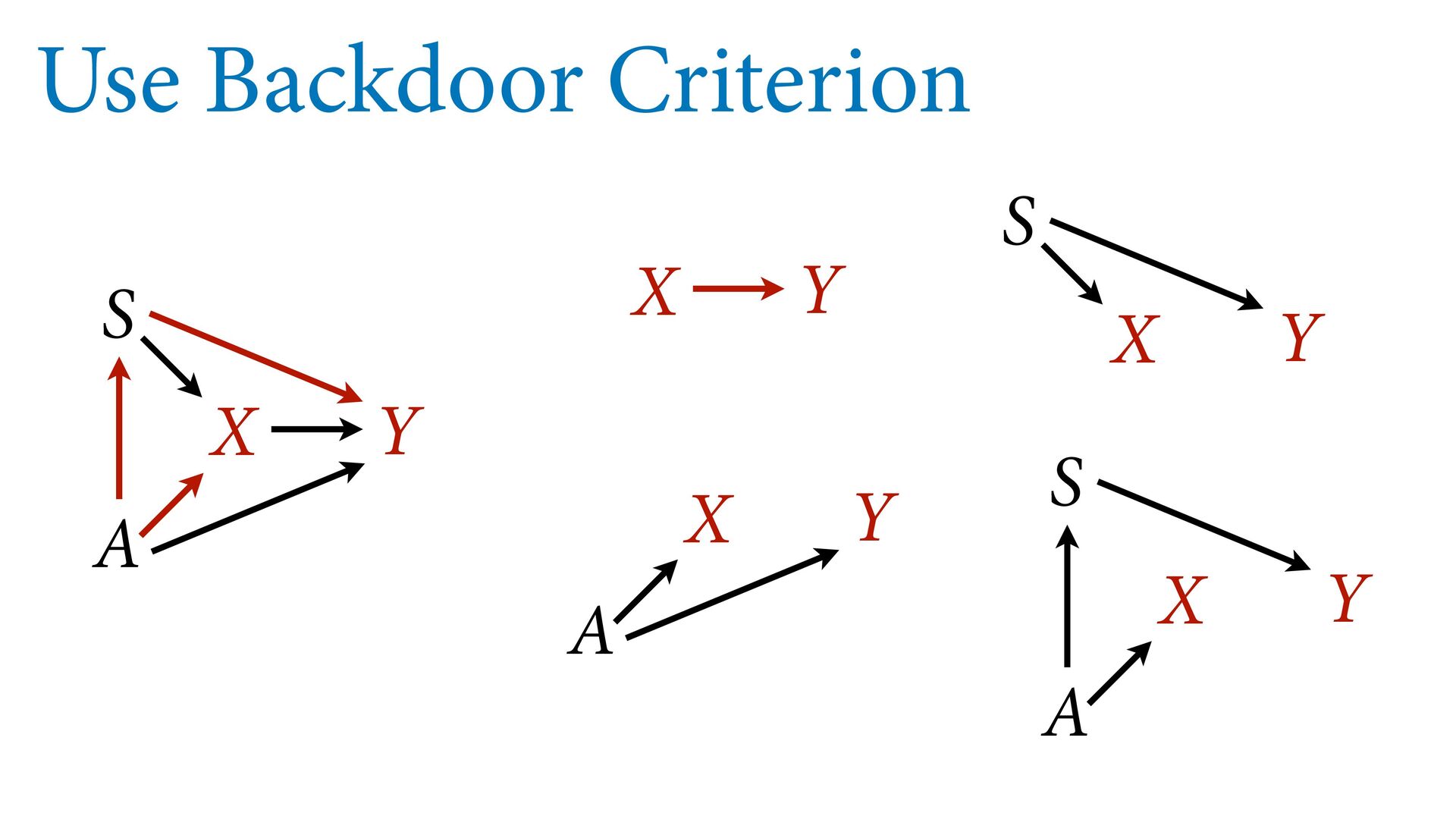
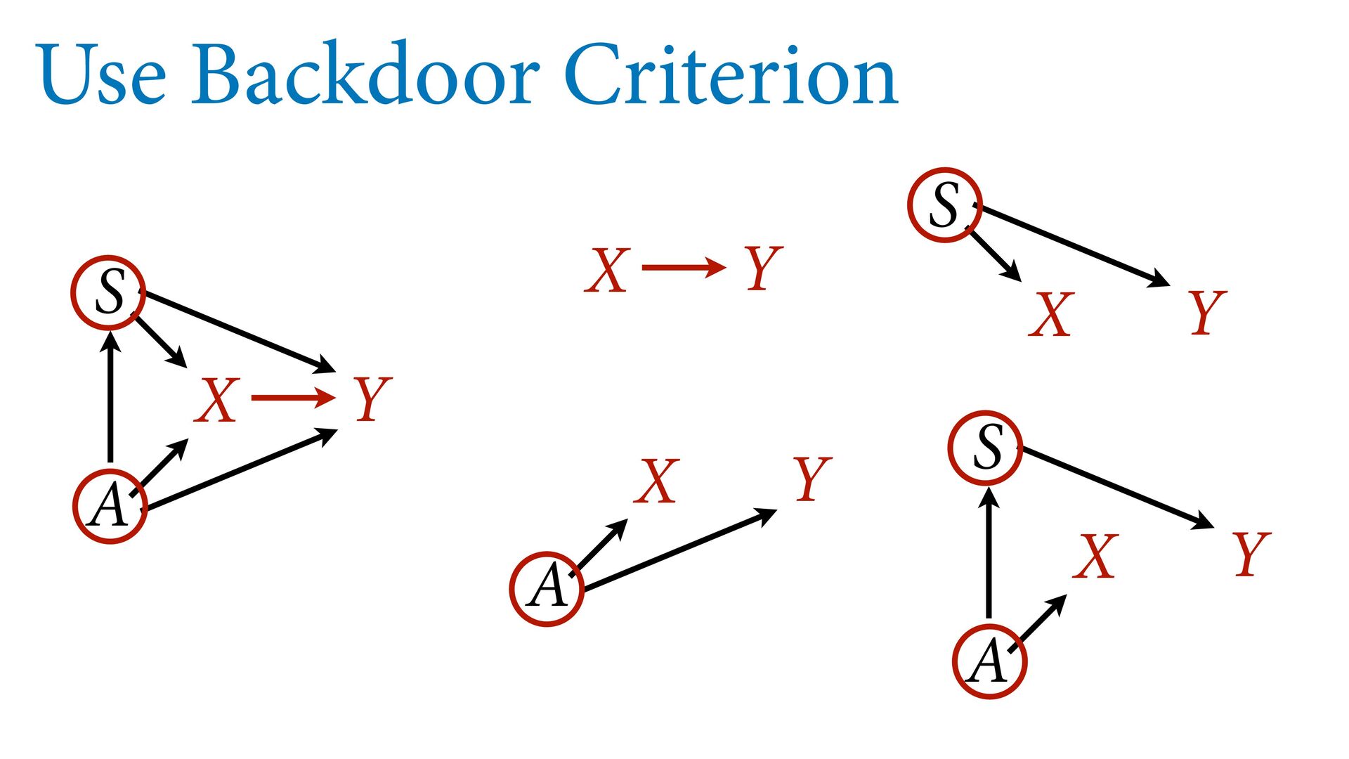
30. Backdoor Criterion Backdoor Criterion: Rule to find a set of variables to stratify (condition) by to yield P(Y|do(X)) (1) Identify all paths connection the treatment (X) to the outcome (Y) (2) Paths with arrows entering X are backdoor paths (non-causal paths)
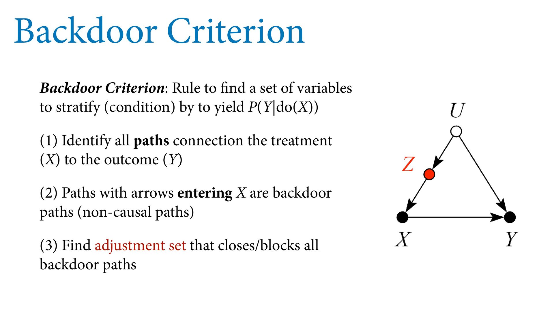
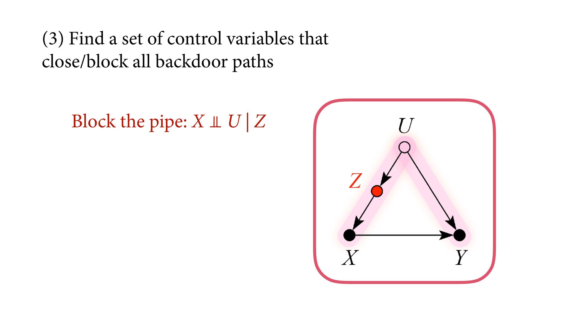
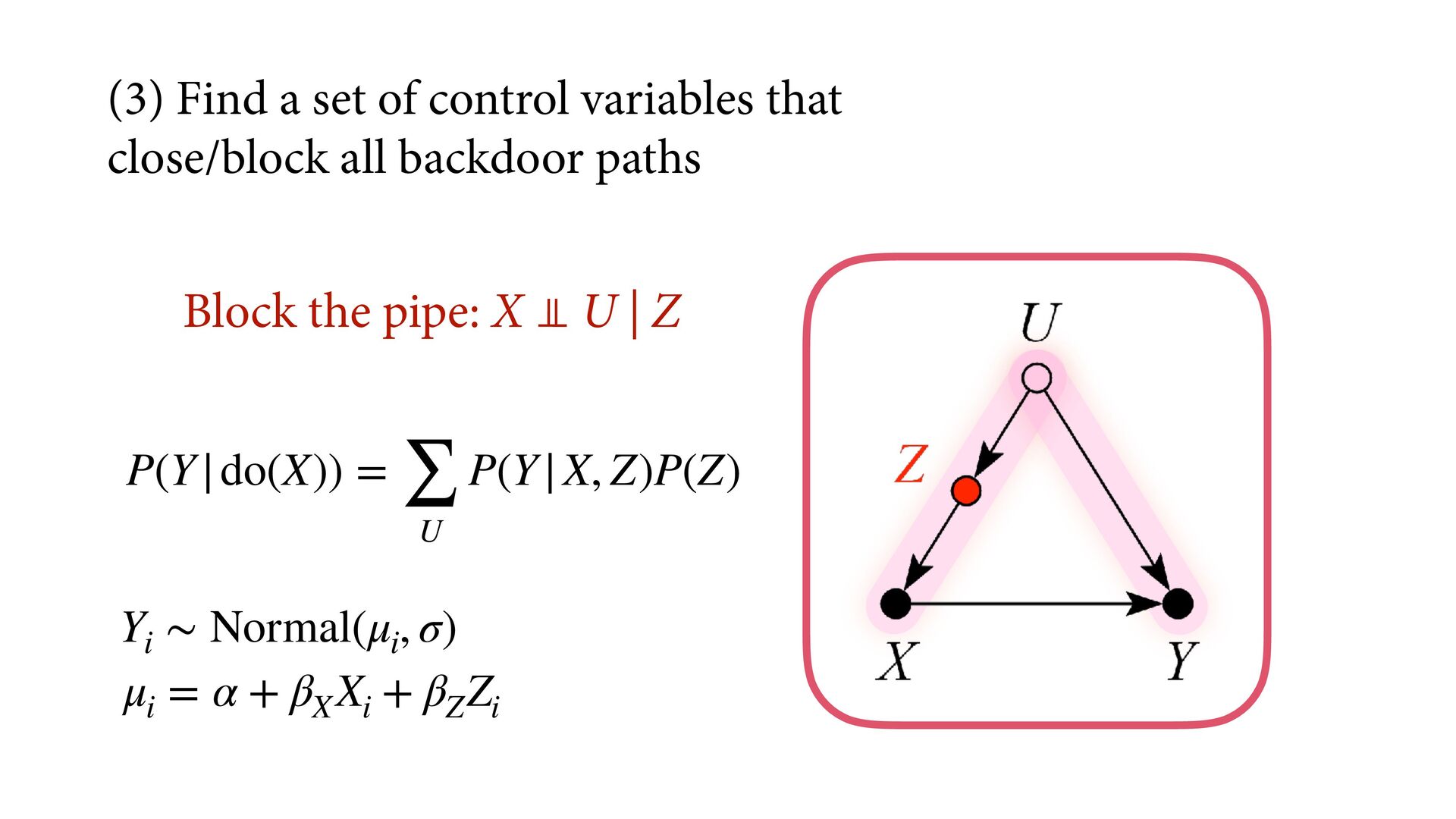
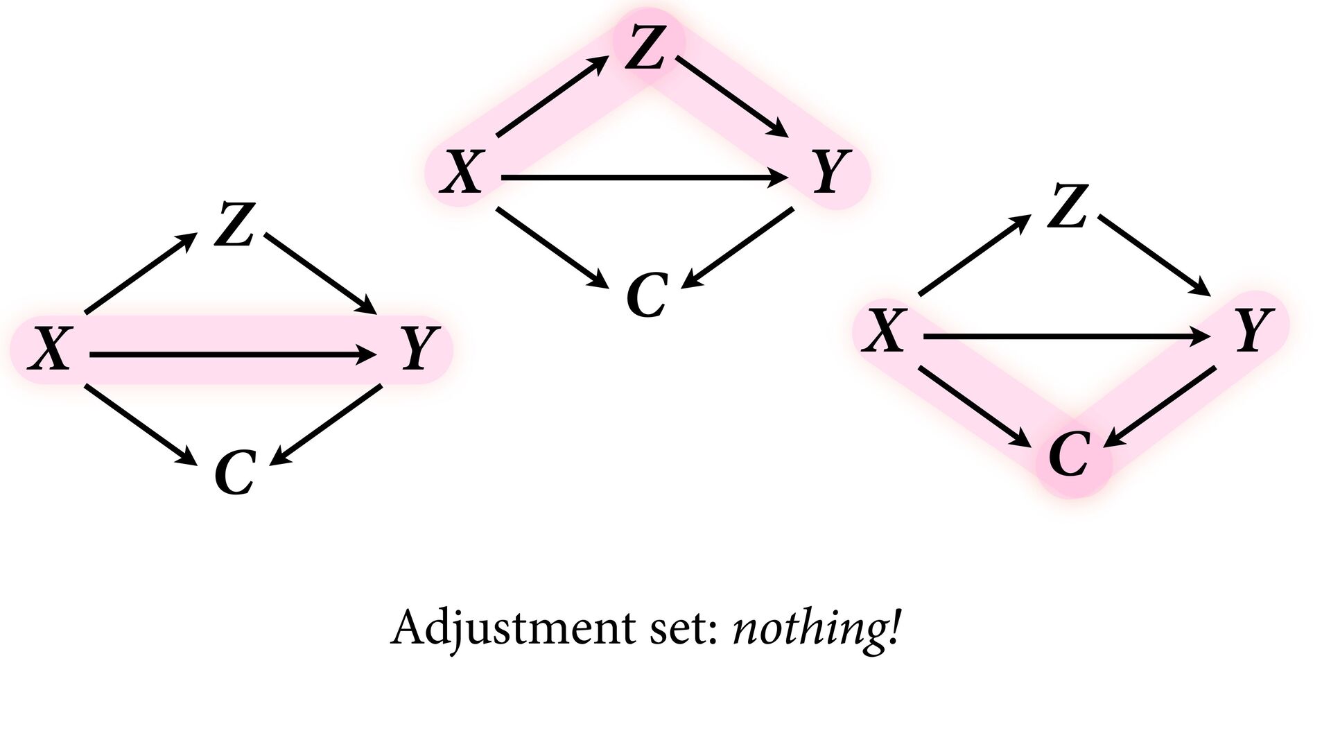
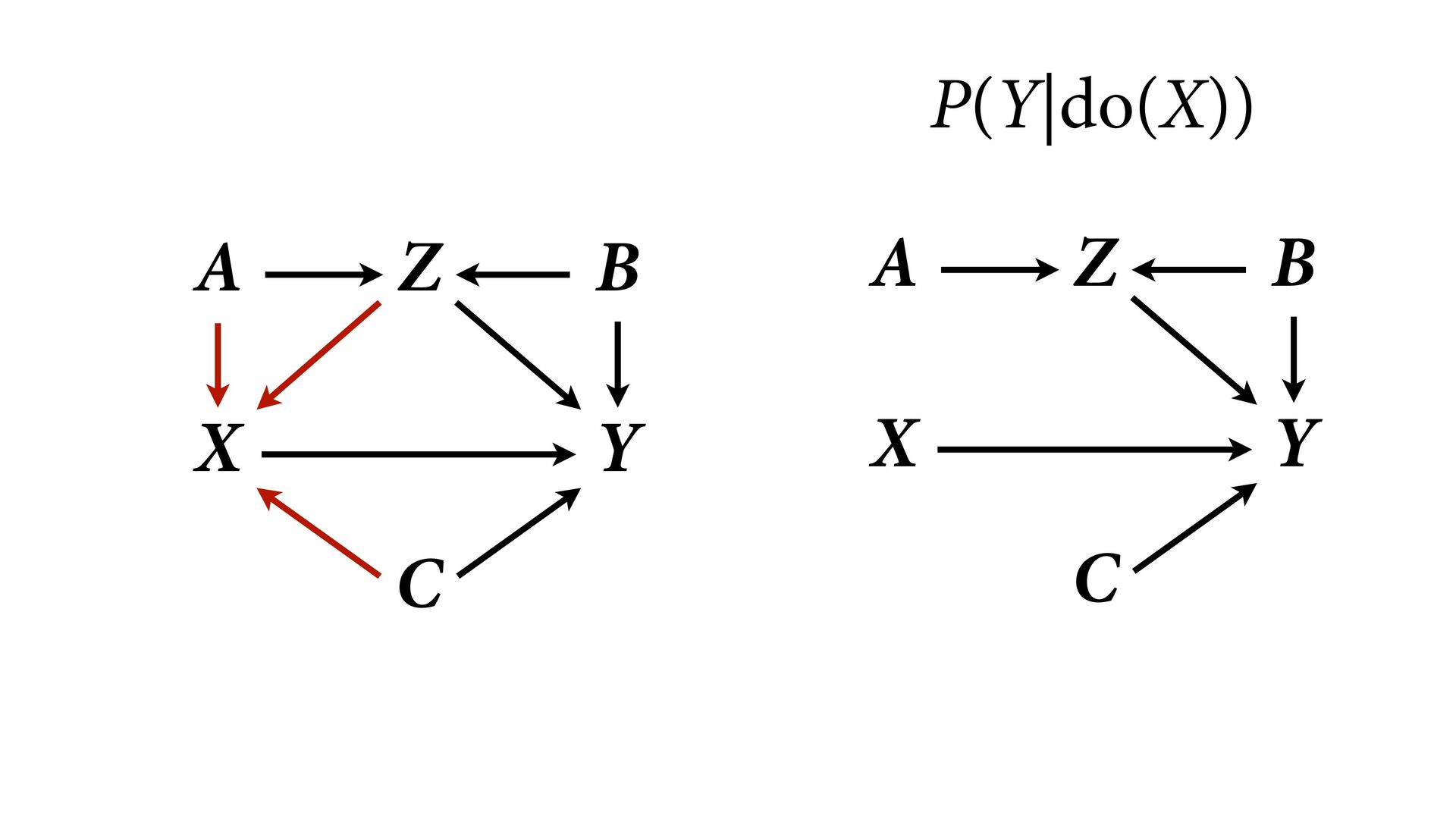
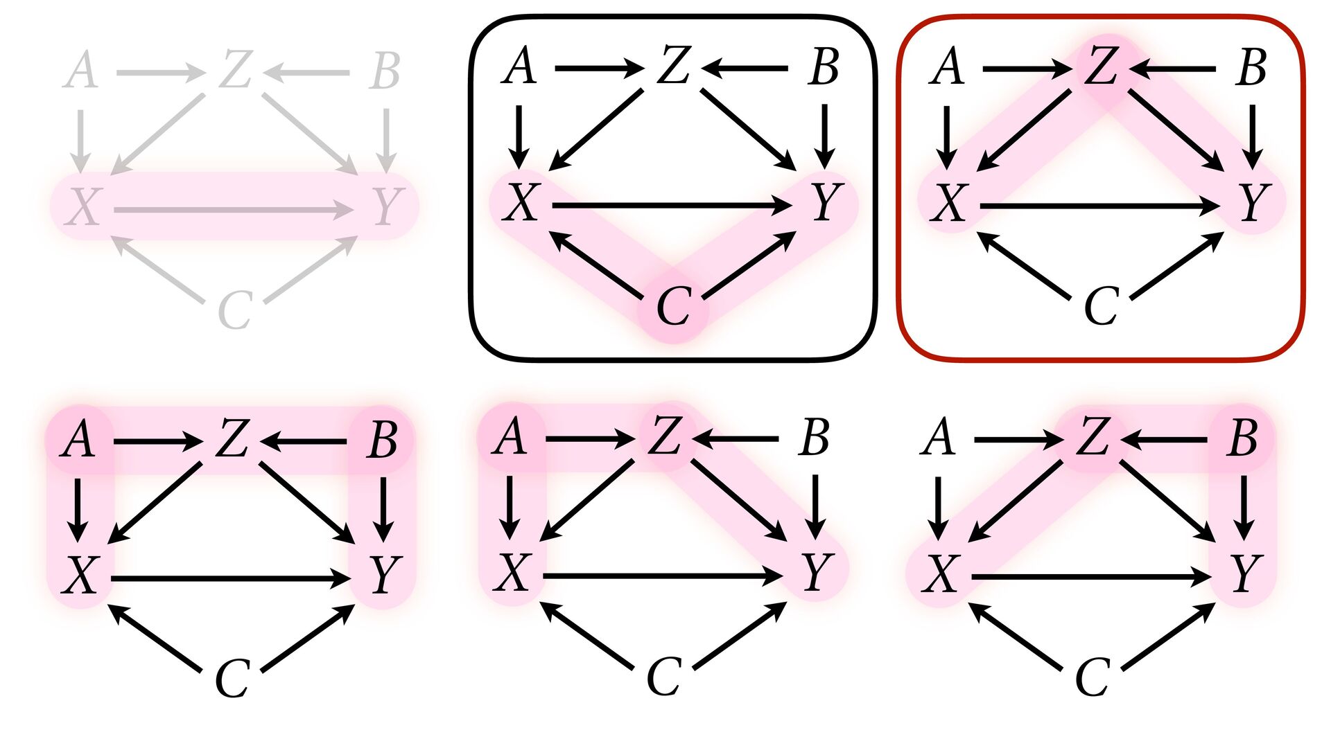
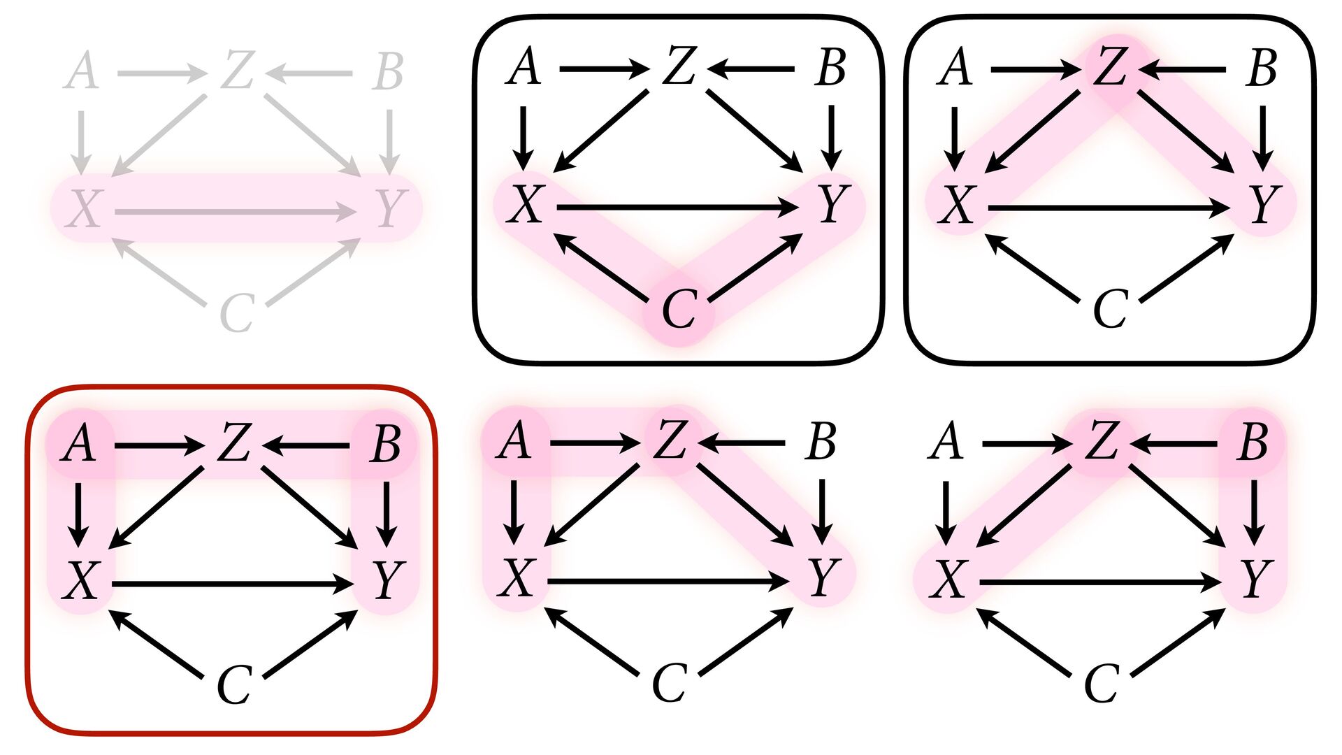
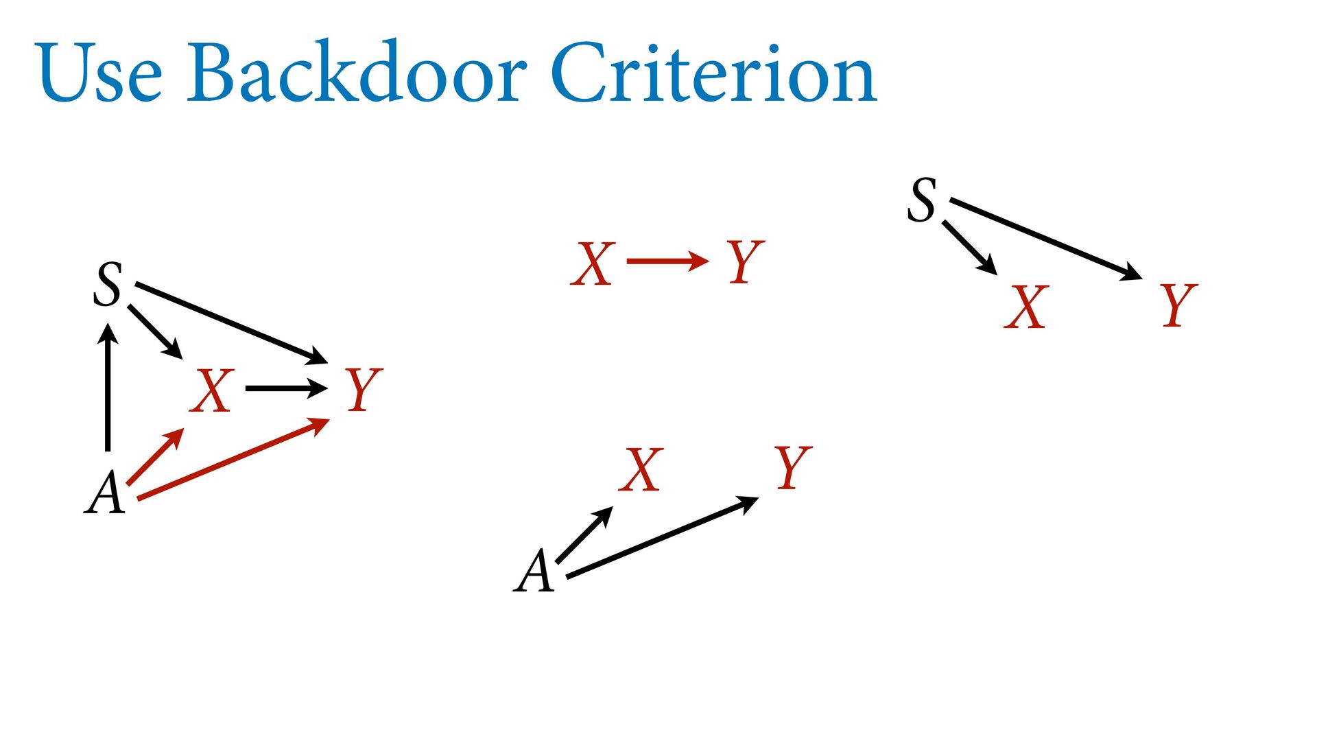
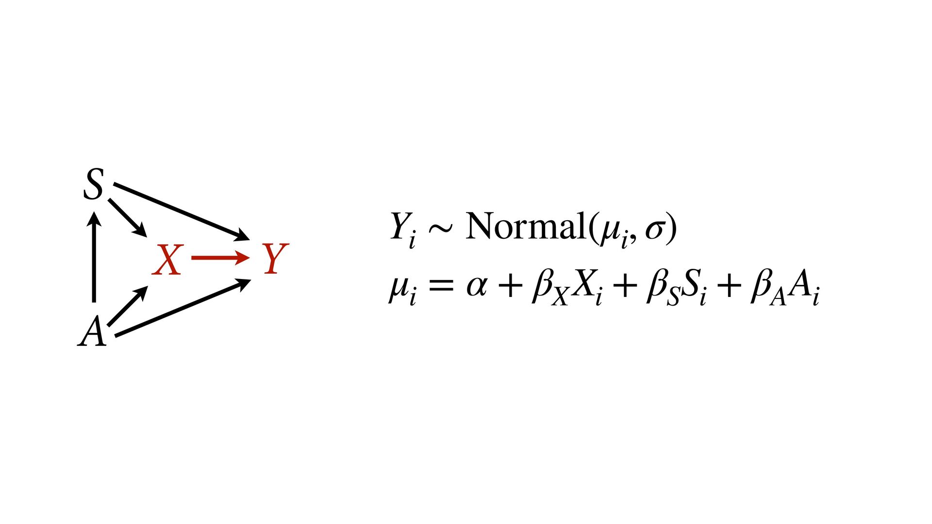
31. Backdoor Criterion Backdoor Criterion: Rule to find a set of variables to stratify (condition) by to yield P(Y|do(X)) (1) Identify all paths connection the treatment (X) to the outcome (Y) (2) Paths with arrows entering X are backdoor paths (non-causal paths) (3) Find adjustment set that closes/blocks all backdoor paths
32. (1) Identify all paths connection the treatment (X) to the outcome (Y)
33. (2) Paths with arrows entering X are backdoor paths (non-causal paths)
34. (3) Find a set of control variables that close/block all backdoor paths Block the pipe: X ⫫ U | Z
35. (3) Find a set of control variables that close/block all backdoor paths P(Y|do(X)) = ∑ U P(Y|X, Z)P(Z) μ i = α + β X X i + β Z Z i Y i ∼ Normal(μ i , σ) Block the pipe: X ⫫ U | Z
36. X Y List all the paths connecting X and Y. Which need to be closed to estimate effect of X on Y? C Z
37. X Y List all the paths connecting X and Y. Which need to be closed to estimate effect of X on Y? C Z X Y C Z X Y C Z
38. X Y C Z X Y C Z X Y C Z Adjustment set: nothing!
39. X Y Z B List all the paths connecting X and Y. Which need to be closed to estimate effect of X on Y? A C
41. X Y Z B A C P(Y|do(X)) X Y Z B A C
42. X Y Z B A C P(Y|do(X)) X Y Z B A C
43. X Y Z B A C X Y Z B A C X Y Z B A C X Y Z B A C X Y Z B A C X Y Z B A C
44. X Y Z B A C X Y Z B A C X Y Z B A C X Y Z B A C X Y Z B A C X Y Z B A C
45. X Y Z B A C X Y Z B A C X Y Z B A C X Y Z B A C X Y Z B A C X Y Z B A C
46. X Y Z B A C X Y Z B A C X Y Z B A C X Y Z B A C X Y Z B A C X Y Z B A C
47. X Y Z B A C X Y Z B A C X Y Z B A C X Y Z B A C X Y Z B A C X Y Z B A C
48. X Y Z B A C X Y Z B A C X Y Z B A C Adjustment set: C, Z, and either A or B (B is better choice)
49. www.dagitty.net
50. Backdoor Criterion Backdoor Criterion: Rule to find adjustment set to yield P(Y|do(X))
51. Backdoor Criterion Backdoor Criterion: Rule to find adjustment set to yield P(Y|do(X)) Beware non-causal paths that you open while closing other paths!
52. Backdoor Criterion Backdoor Criterion: Rule to find adjustment set to yield P(Y|do(X)) Beware non-causal paths that you open while closing other paths! More than backdoors:
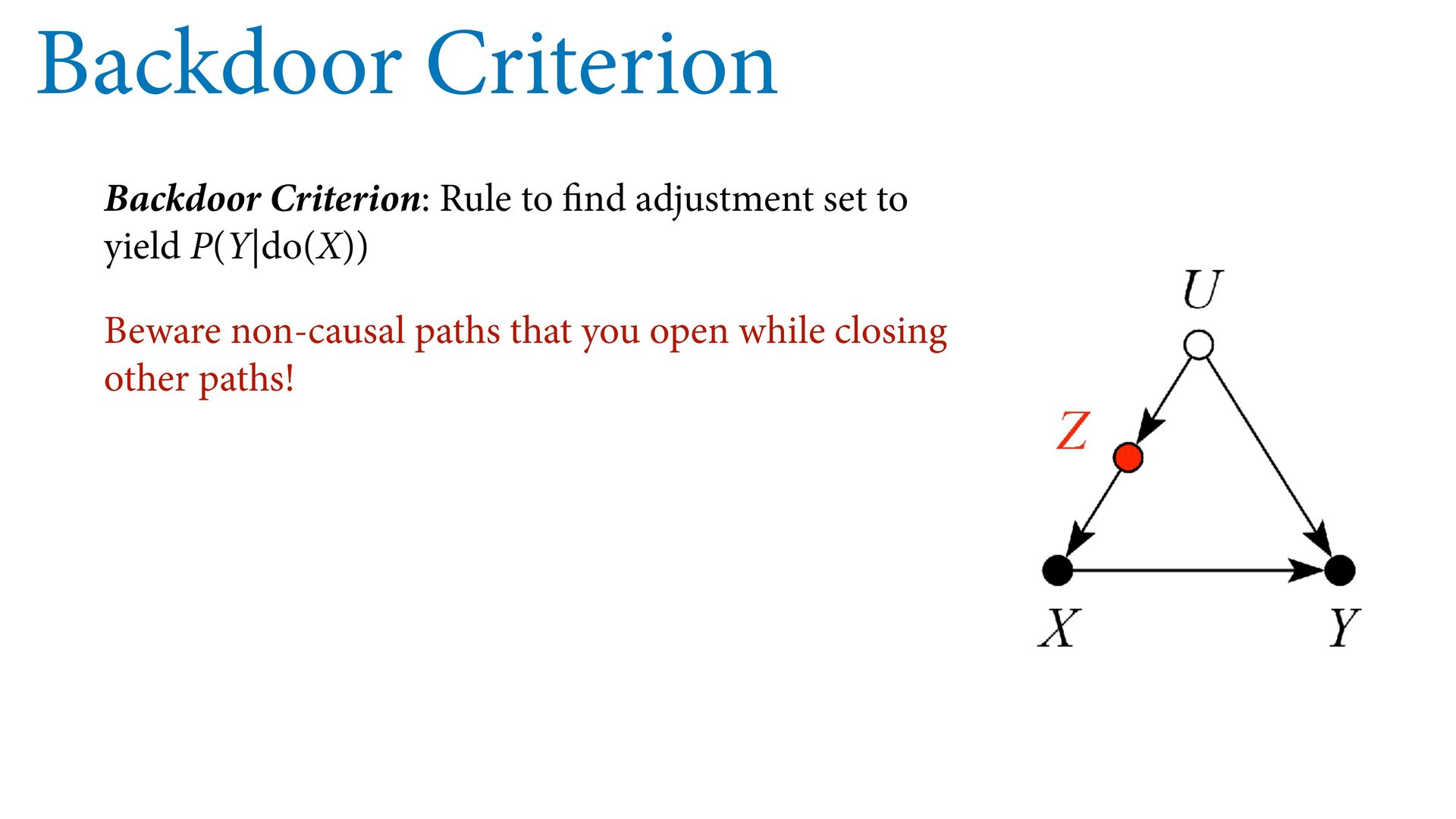
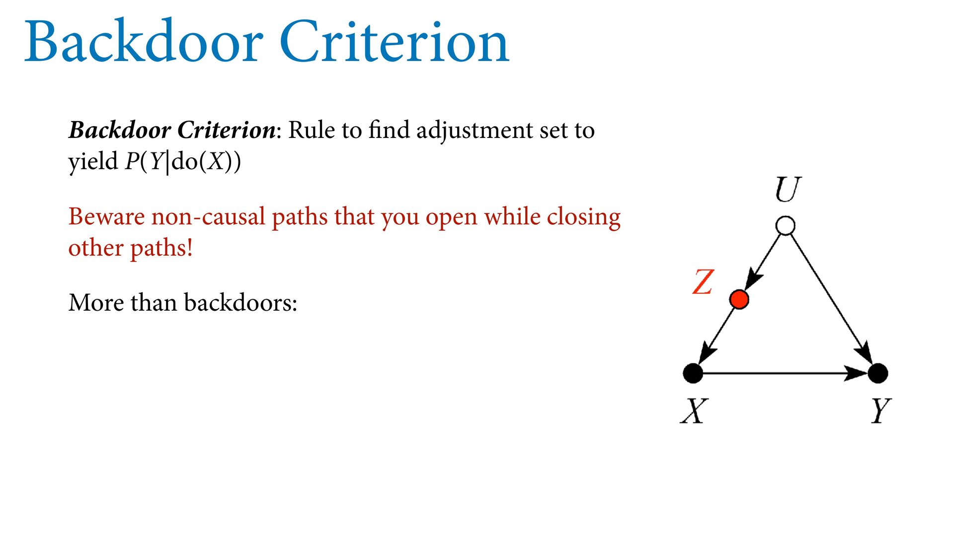
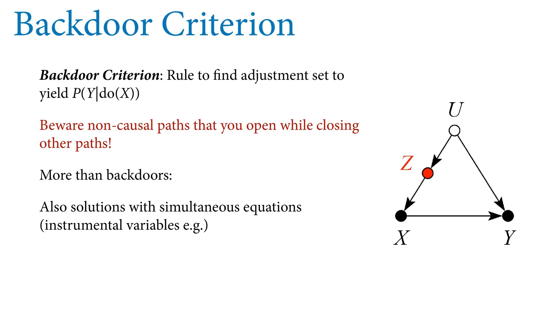
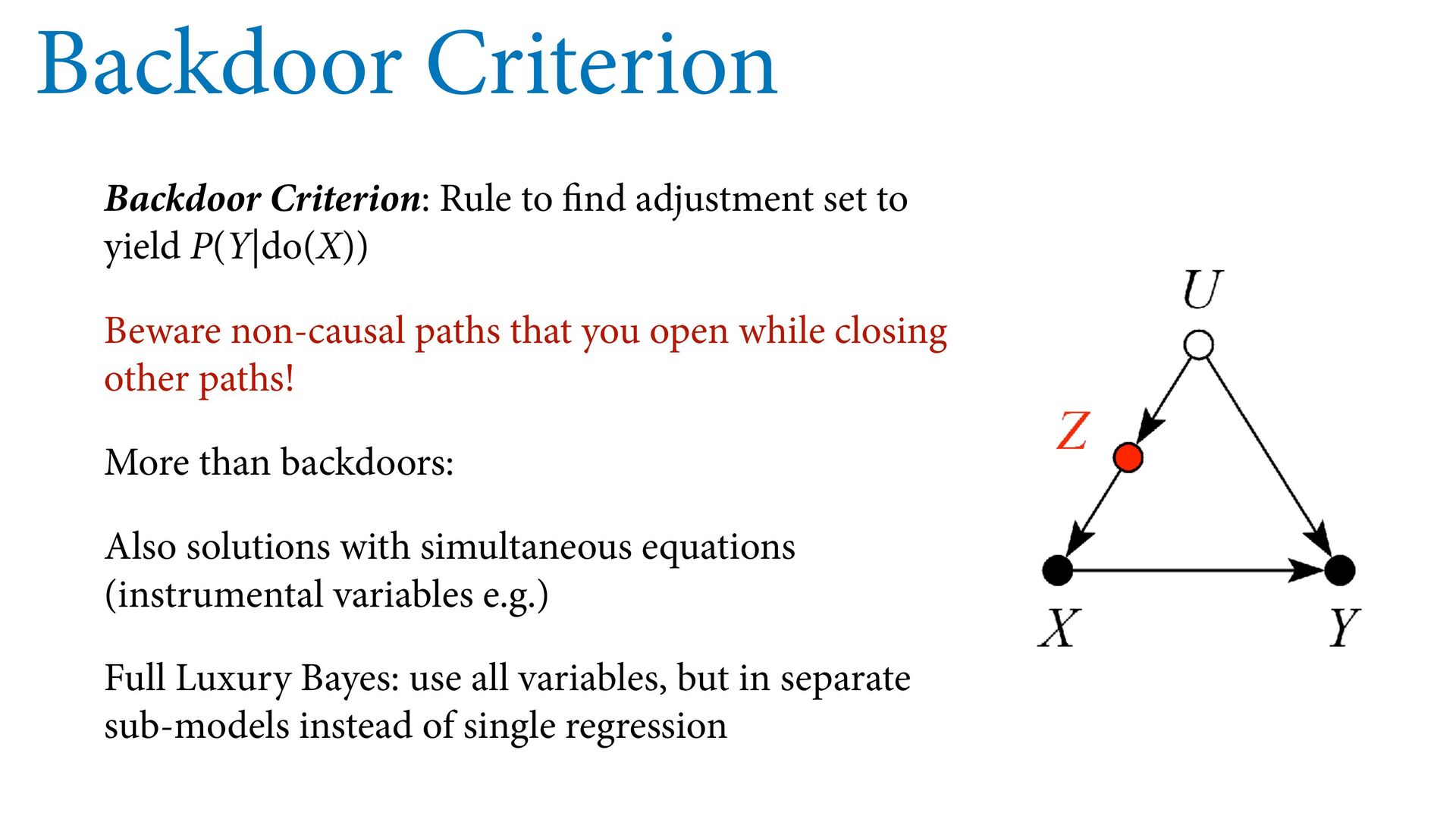
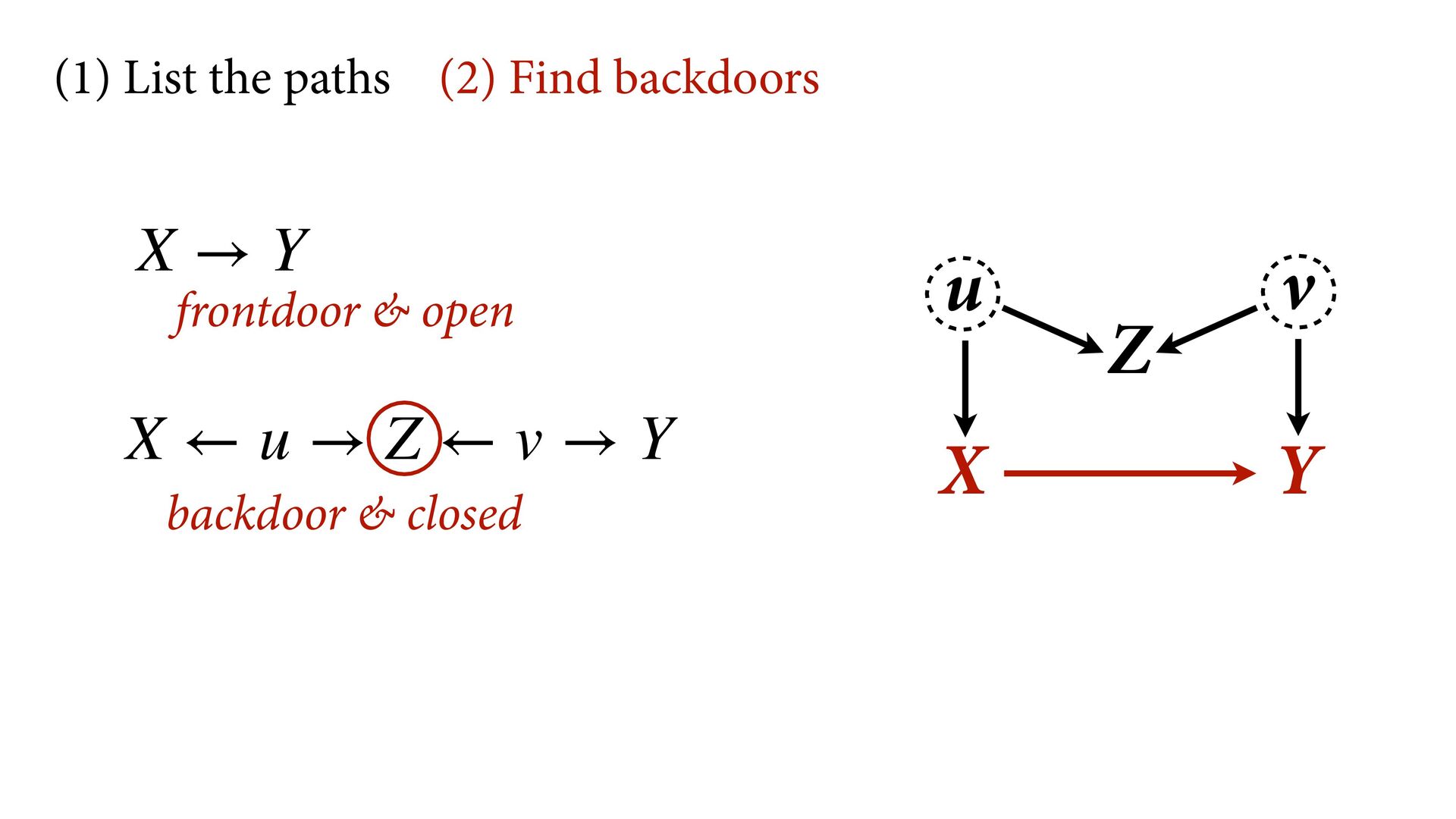
53. Backdoor Criterion Backdoor Criterion: Rule to find adjustment set to yield P(Y|do(X)) Beware non-causal paths that you open while closing other paths! More than backdoors: Also solutions with simultaneous equations (instrumental variables e.g.)
54. Backdoor Criterion Backdoor Criterion: Rule to find adjustment set to yield P(Y|do(X)) Beware non-causal paths that you open while closing other paths! More than backdoors: Also solutions with simultaneous equations (instrumental variables e.g.) Full Luxury Bayes: use all variables, but in separate sub-models instead of single regression
55. PAUSE
56. http://www.blackswanman.com/
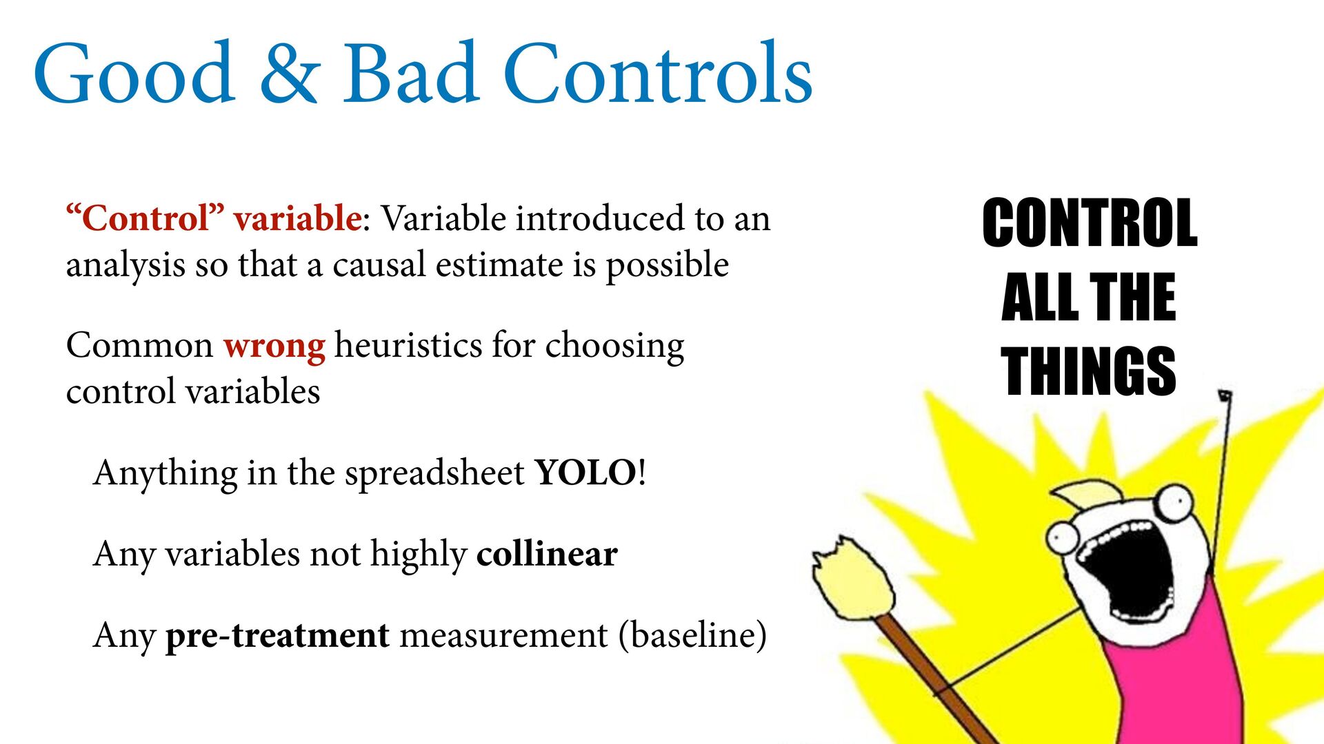
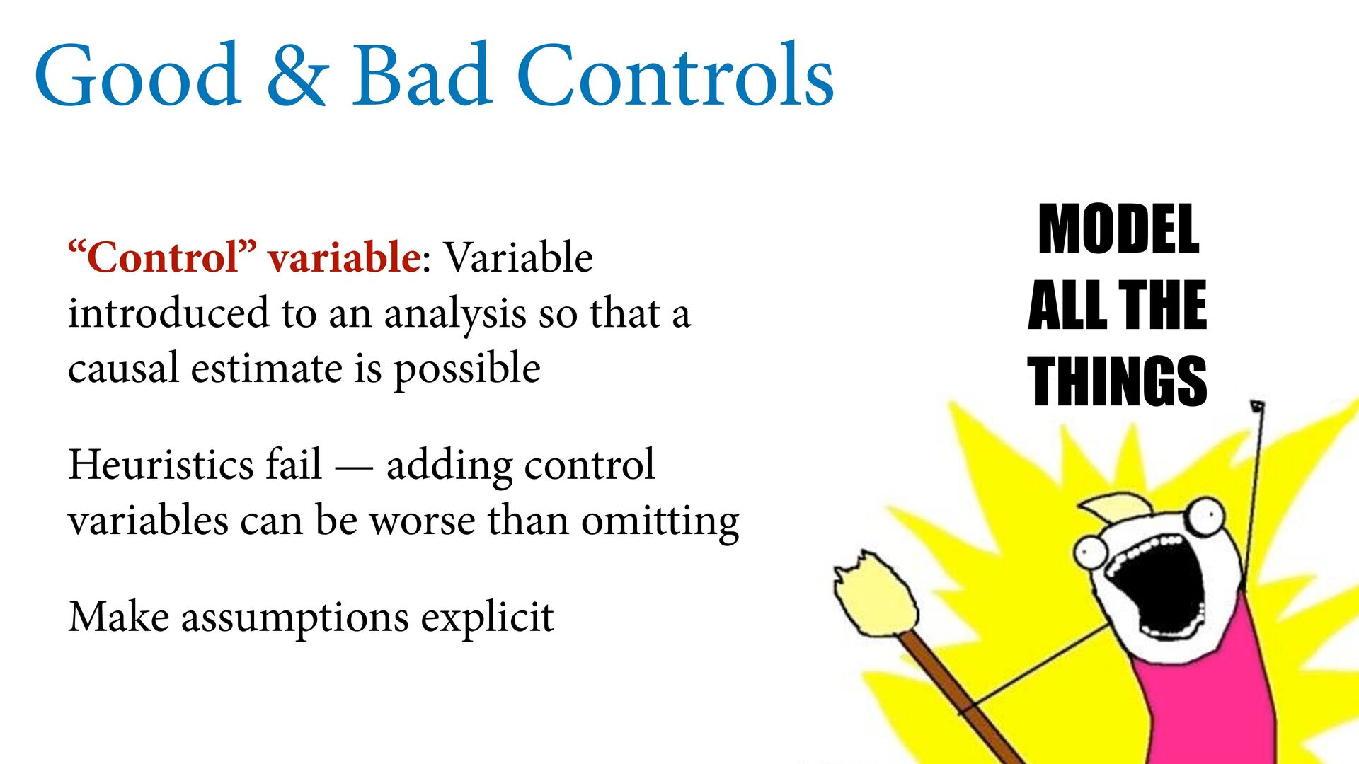
57. Good & Bad Controls “Control” variable: Variable introduced to an analysis so that a causal estimate is possible Common wrong heuristics for choosing control variables Anything in the spreadsheet YOLO! Any variables not highly collinear Any pre-treatment measurement (baseline) CONTROL ALL THE THINGS
58. X Cinelli, Forney, Pearl 2021 A Crash Course in Good and Bad Controls Y
59. X Y u v Z Cinelli, Forney, Pearl 2021 A Crash Course in Good and Bad Controls unobserved
60. X Y u v Z Cinelli, Forney, Pearl 2021 A Crash Course in Good and Bad Controls Health
 person 1 Health person 2 Hobbies person 1 Hobbies person 2 Friends
61. X Y u v Z (1) List the paths
62. X Y u v Z (1) List the paths X → Y
63. X Y u v Z (1) List the paths X → Y X ← u → Z ← v → Y
64. X Y u v Z (1) List the paths X → Y X ← u → Z ← v → Y frontdoor & open backdoor & closed (2) Find backdoors
65. X Y u v Z (1) List the paths X → Y X ← u → Z ← v → Y frontdoor & open backdoor & closed (2) Find backdoors
66. X Y u v Z (1) List the paths X → Y X ← u → Z ← v → Y frontdoor & open backdoor & closed (2) Find backdoors (3) Close backdoors
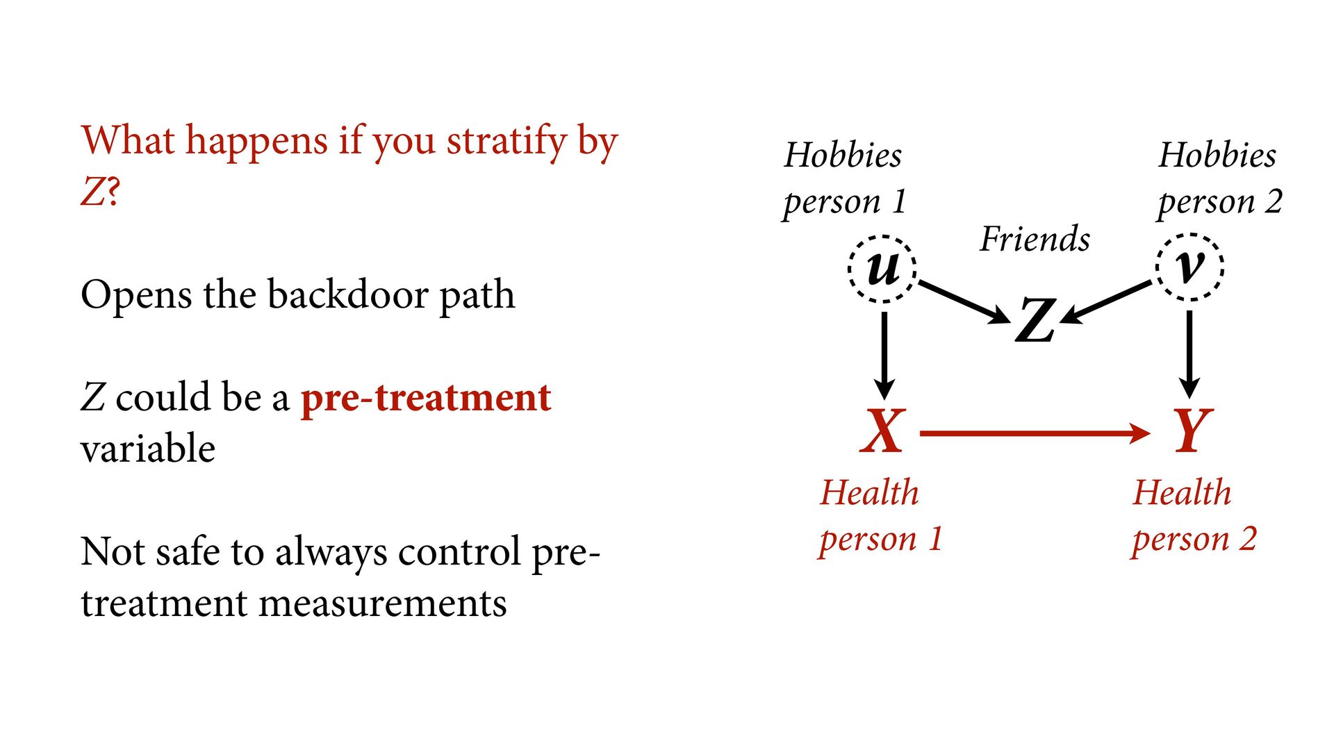
67. X Y u v Z What happens if you stratify by Z? Opens the backdoor path Z could be a pre-treatment variable Not safe to always control pre- treatment measurements Health
 person 1 Health person 2 Hobbies person 1 Hobbies person 2 Friends
68. X Y Z u
69. X Y Z u Win lottery Lifespan Happiness Contextual confounds
70. X Y Z u X → Z → Y X → Z ← u → Y No backdoor, no need to control for Z
71. X Y Z u f <- function(n=100,bXZ=1,bZY=1) { X <- rnorm(n) u <- rnorm(n) Z <- rnorm(n, bXZ*X + u) Y <- rnorm(n, bZY*Z + u ) bX <- coef( lm(Y ~ X) )['X'] bXZ <- coef( lm(Y ~ X + Z) )['X'] return( c(bX,bXZ) ) } sim <- mcreplicate( 1e4 , f() , mc.cores=8 ) dens( sim[1,] , lwd=3 , xlab="posterior mean" ) dens( sim[2,] , lwd=3 , col=2 , add=TRUE ) 1 1 1 1
72. X Y Z u -1.0 0.0 0.5 1.0 1.5 2.0 0.0 1.0 2.0 posterior mean Density f <- function(n=100,bXZ=1,bZY=1) { X <- rnorm(n) u <- rnorm(n) Z <- rnorm(n, bXZ*X + u) Y <- rnorm(n, bZY*Z + u ) bX <- coef( lm(Y ~ X) )['X'] bXZ <- coef( lm(Y ~ X + Z) )['X'] return( c(bX,bXZ) ) } sim <- mcreplicate( 1e4 , f() , mc.cores=8 ) dens( sim[1,] , lwd=3 , xlab="posterior mean" ) dens( sim[2,] , lwd=3 , col=2 , add=TRUE ) Y ~ X correct Y ~ X + Z wrong 1 1 1 1
73. X Y Z u Y ~ X correct Y ~ X + Z wrong Change bZY to zero f <- function(n=100,bXZ=1,bZY=1) { X <- rnorm(n) u <- rnorm(n) Z <- rnorm(n, bXZ*X + u) Y <- rnorm(n, bZY*Z + u ) bX <- coef( lm(Y ~ X) )['X'] bXZ <- coef( lm(Y ~ X + Z) )['X'] return( c(bX,bXZ) ) } sim <- mcreplicate( 1e4 , f(bZY=0) , mc.cores=8 ) dens( sim[1,] , lwd=3 , xlab="posterior mean" ) dens( sim[2,] , lwd=3 , col=2 , add=TRUE ) -1.0 -0.5 0.0 0.5 0.0 1.0 2.0 posterior mean Density 1 0 1 1
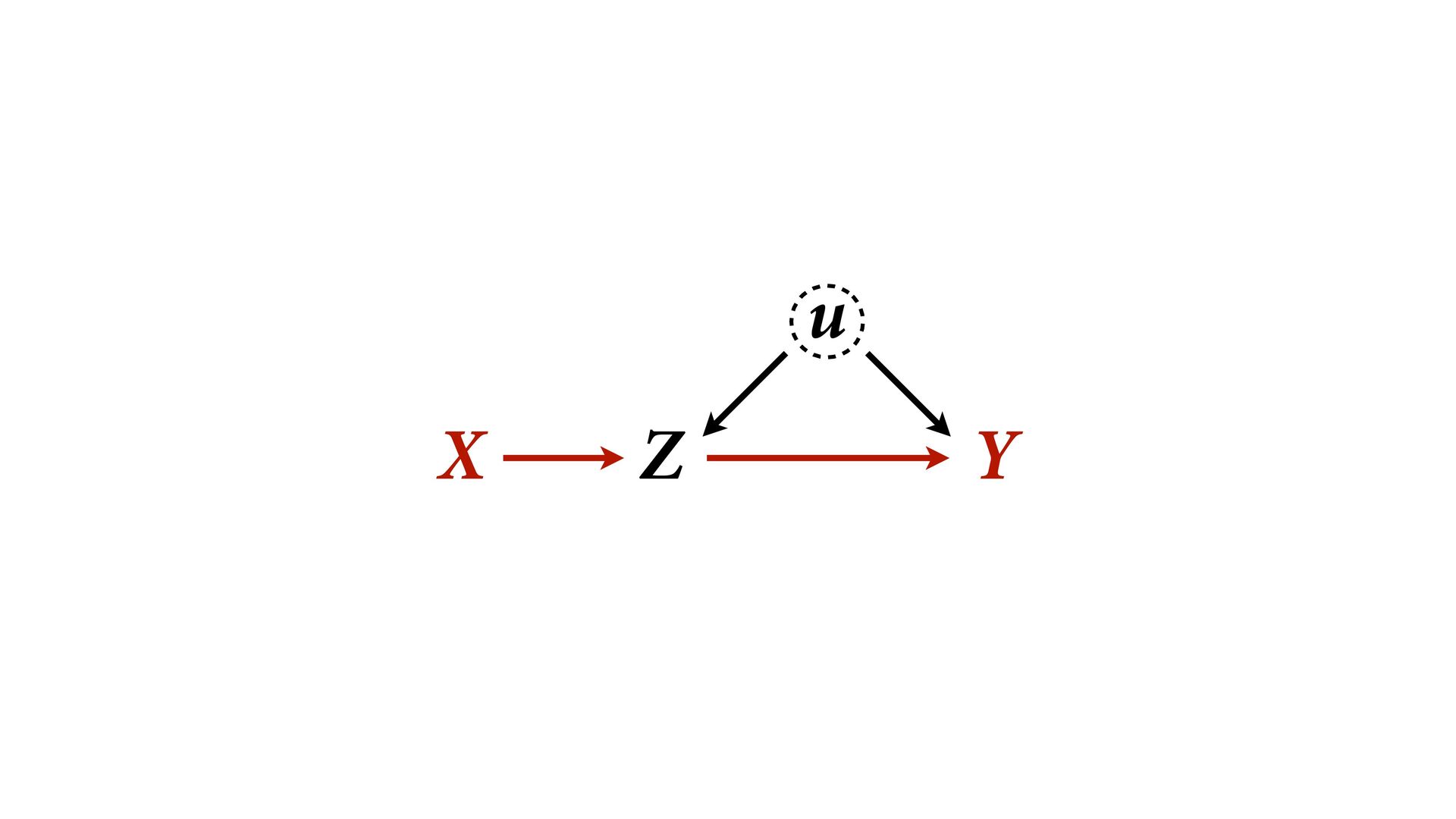
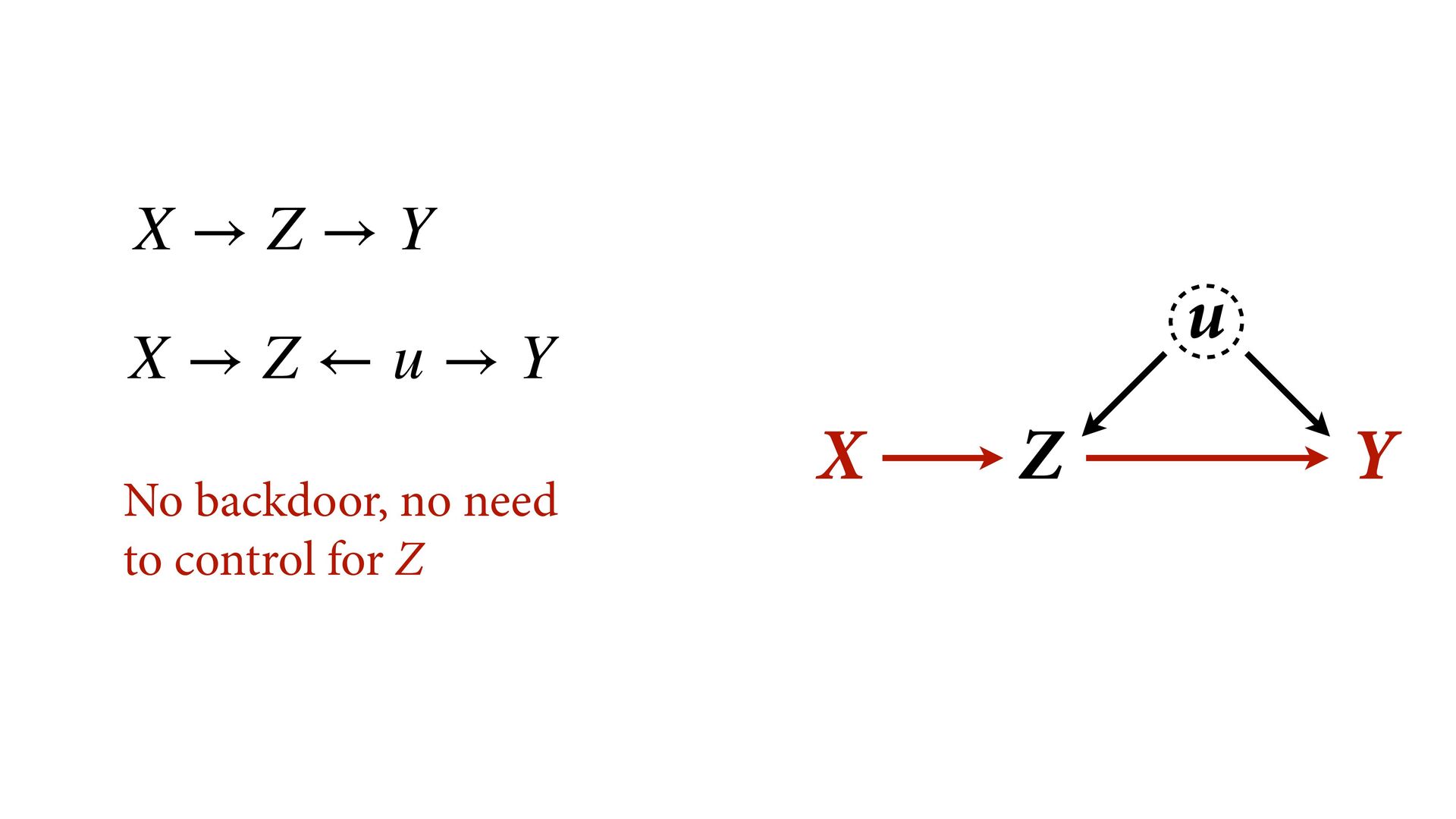
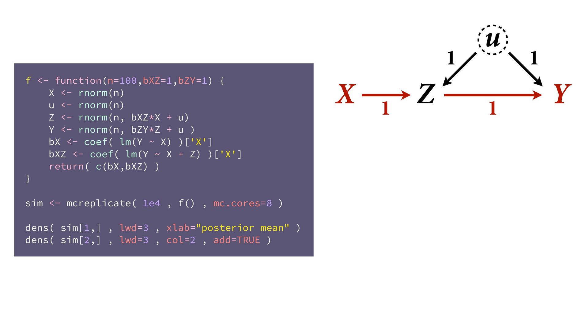
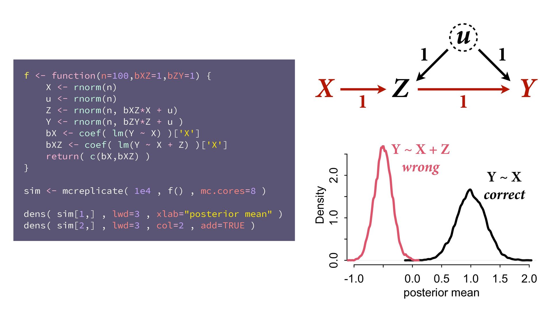
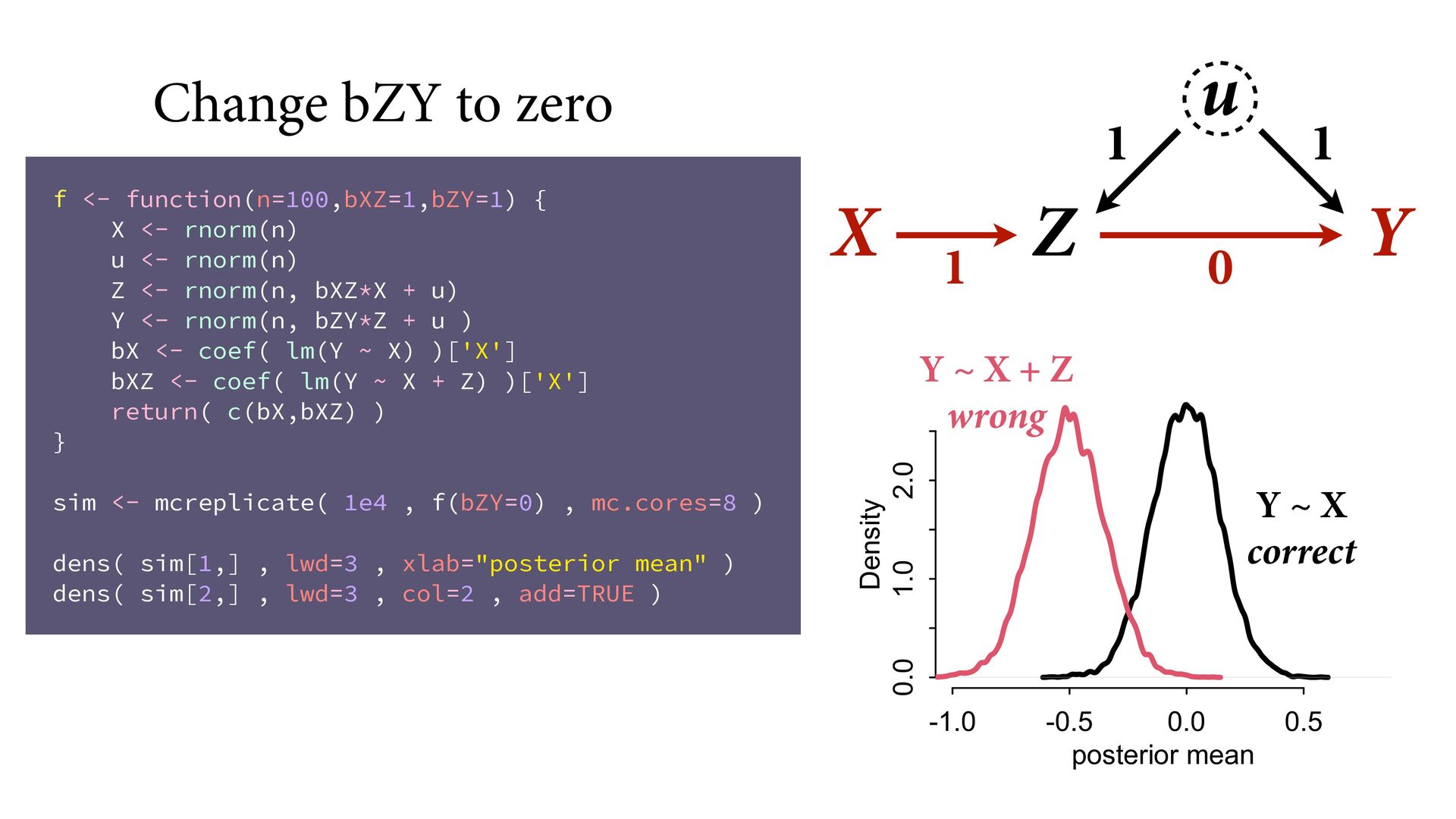
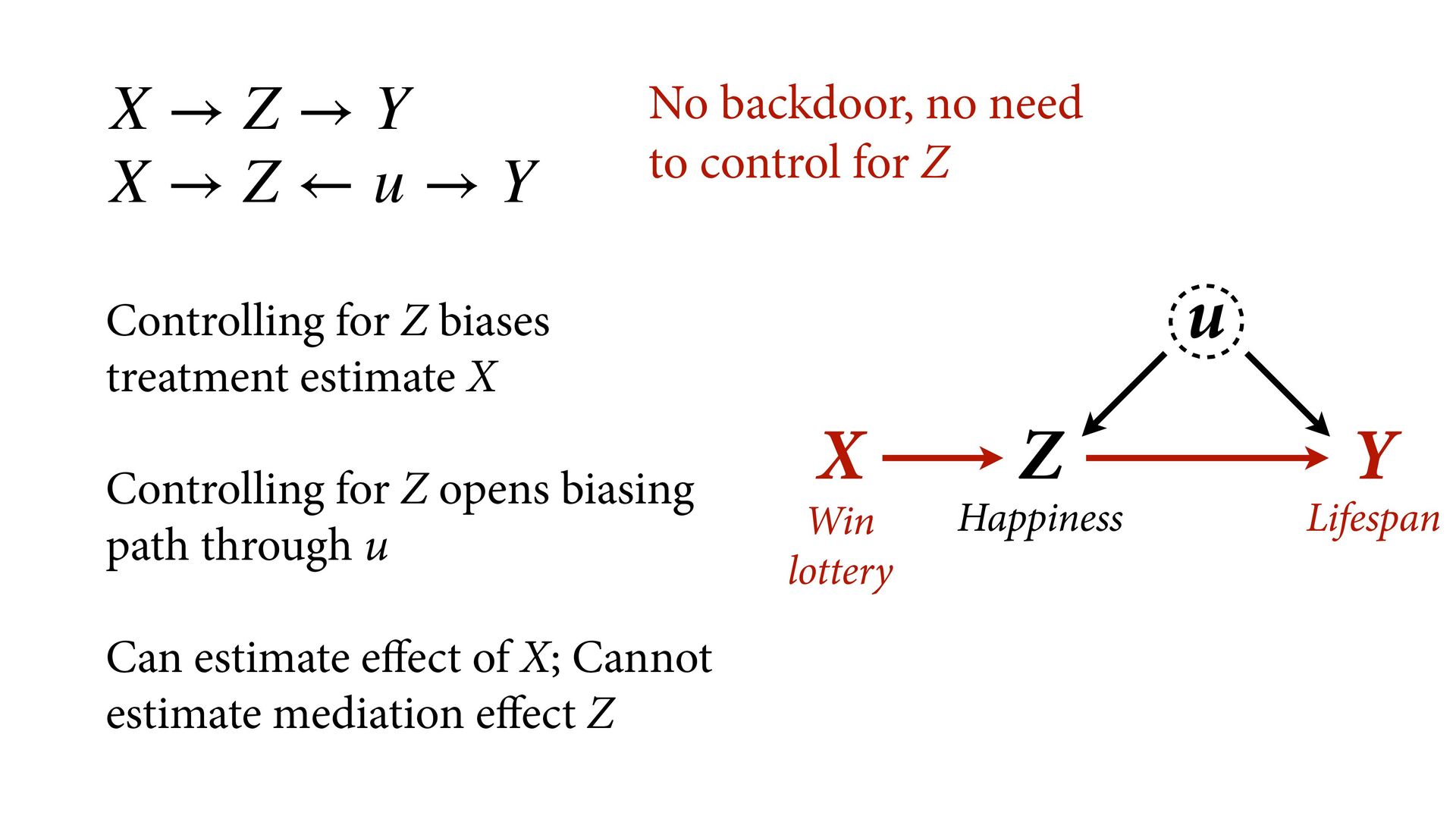
74. X Y Z u X → Z → Y X → Z ← u → Y No backdoor, no need to control for Z Controlling for Z biases treatment estimate X Controlling for Z opens biasing path through u Can estimate effect of X; Cannot estimate mediation effect Z Win lottery Lifespan Happiness
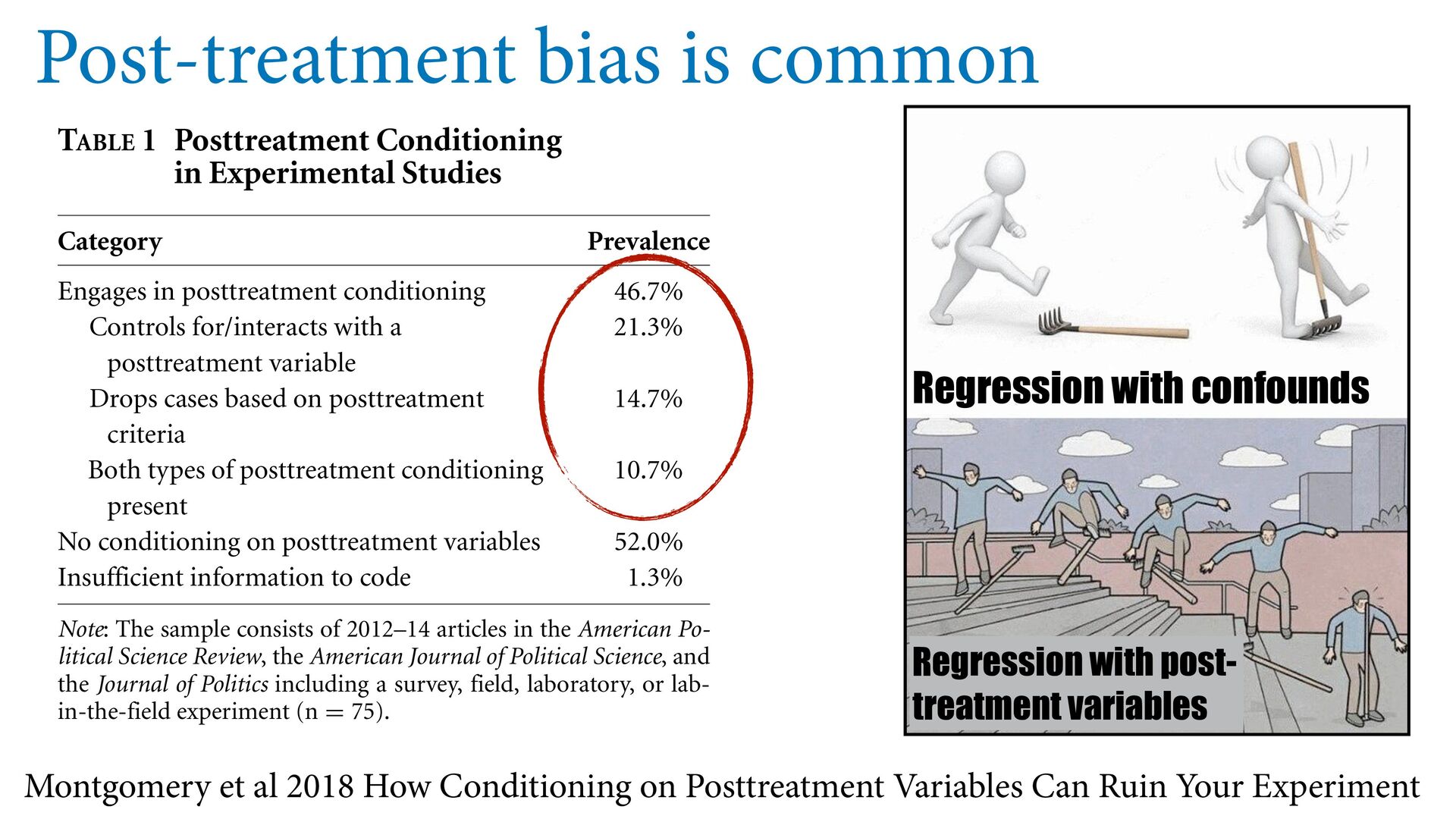
75. Post-treatment bias is common IMENTS 761 - s; g s, d 6; - s o t - h. - - e - t m TABLE 1 Posttreatment Conditioning in Experimental Studies Category Prevalence Engages in posttreatment conditioning 46.7% Controls for/interacts with a posttreatment variable 21.3% Drops cases based on posttreatment criteria 14.7% Both types of posttreatment conditioning present 10.7% No conditioning on posttreatment variables 52.0% Insufficient information to code 1.3% Note: The sample consists of 2012–14 articles in the American Po- litical Science Review, the American Journal of Political Science, and the Journal of Politics including a survey, field, laboratory, or lab- in-the-field experiment (n = 75). avoid posttreatment bias. In many cases, the usefulness Montgomery et al 2018 How Conditioning on Posttreatment Variables Can Ruin Your Experiment Regression with confounds Regression with post- treatment variables
76. X Y Z Do not touch the collider!
77. X Y Z u Colliders not always so obvious
78. X Y Z u education values income family
79. X Y Z “Case-control bias”
80. X Y Z “Case-control bias” Education Occupation Income
81. X Y Z “Case-control bias” f <- function(n=100,bXY=1,bYZ=1) { X <- rnorm(n) Y <- rnorm(n, bXY*X ) Z <- rnorm(n, bYZ*Y ) bX <- coef( lm(Y ~ X) )['X'] bXZ <- coef( lm(Y ~ X + Z) )['X'] return( c(bX,bXZ) ) } sim <- mcreplicate( 1e4 , f() , mc.cores=8 ) dens( sim[1,] , lwd=3 , xlab="posterior mean" ) dens( sim[2,] , lwd=3 , col=2 , add=TRUE ) 0.0 0.5 1.0 1.5 0 1 2 3 4 5 posterior mean Density Y ~ X correct Y ~ X + Z wrong 1 1
82. X Y Z “Precision parasite” No backdoors But still not good to condition on Z
83. X Y Z “Precision parasite” f <- function(n=100,bZX=1,bXY=1) { Z <- rnorm(n) X <- rnorm(n, bZX*Z ) Y <- rnorm(n, bXY*X ) bX <- coef( lm(Y ~ X) )['X'] bXZ <- coef( lm(Y ~ X + Z) )['X'] return( c(bX,bXZ) ) } sim <- mcreplicate( 1e4 , f(n=50) , mc.cores=8 ) dens( sim[1,] , lwd=3 , xlab="posterior mean" ) dens( sim[2,] , lwd=3 , col=2 , add=TRUE ) 0.6 0.8 1.0 1.2 1.4 0 1 2 3 4 posterior mean Density Y ~ X correct Y ~ X + Z wrong
84. X Y Z u “Bias amplification” X and Y confounded by u Something truly awful happens when we add Z
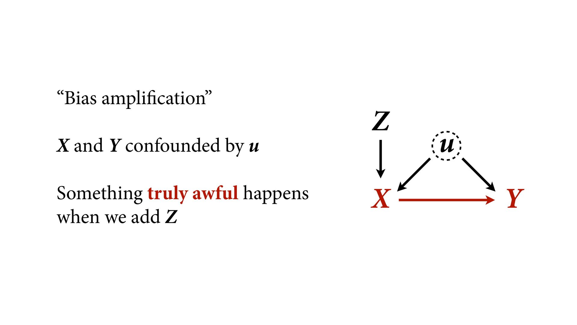
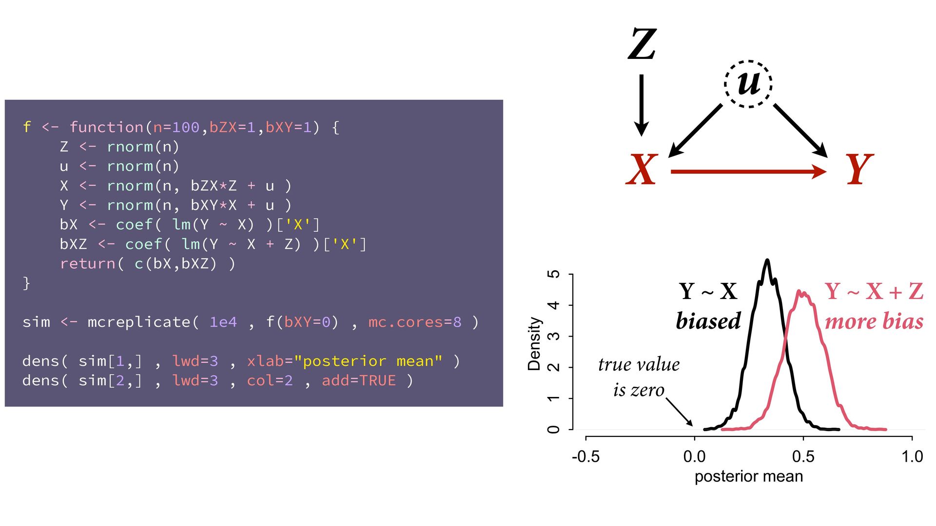
85. f <- function(n=100,bZX=1,bXY=1) { Z <- rnorm(n) u <- rnorm(n) X <- rnorm(n, bZX*Z + u ) Y <- rnorm(n, bXY*X + u ) bX <- coef( lm(Y ~ X) )['X'] bXZ <- coef( lm(Y ~ X + Z) )['X'] return( c(bX,bXZ) ) } sim <- mcreplicate( 1e4 , f(bXY=0) , mc.cores=8 ) dens( sim[1,] , lwd=3 , xlab="posterior mean" ) dens( sim[2,] , lwd=3 , col=2 , add=TRUE ) X Y Z u -0.5 0.0 0.5 1.0 0 1 2 3 4 5 posterior mean Density Y ~ X biased Y ~ X + Z more bias true value is zero
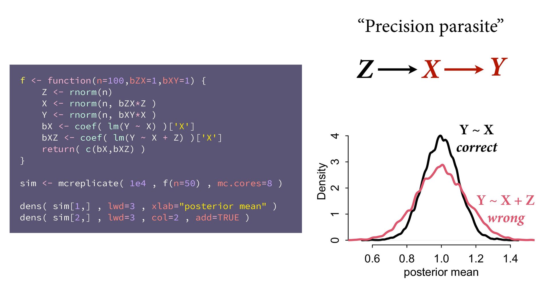
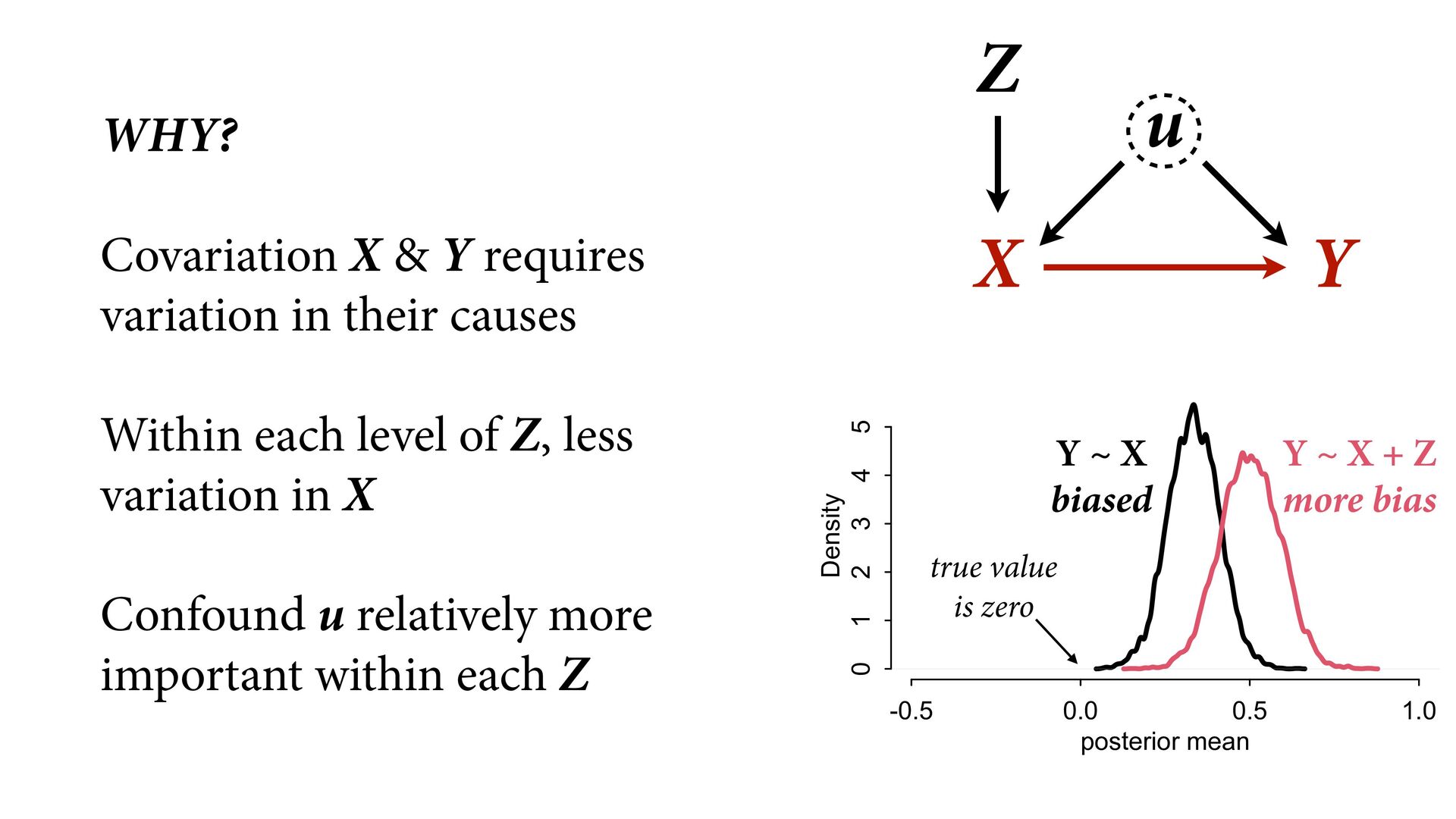
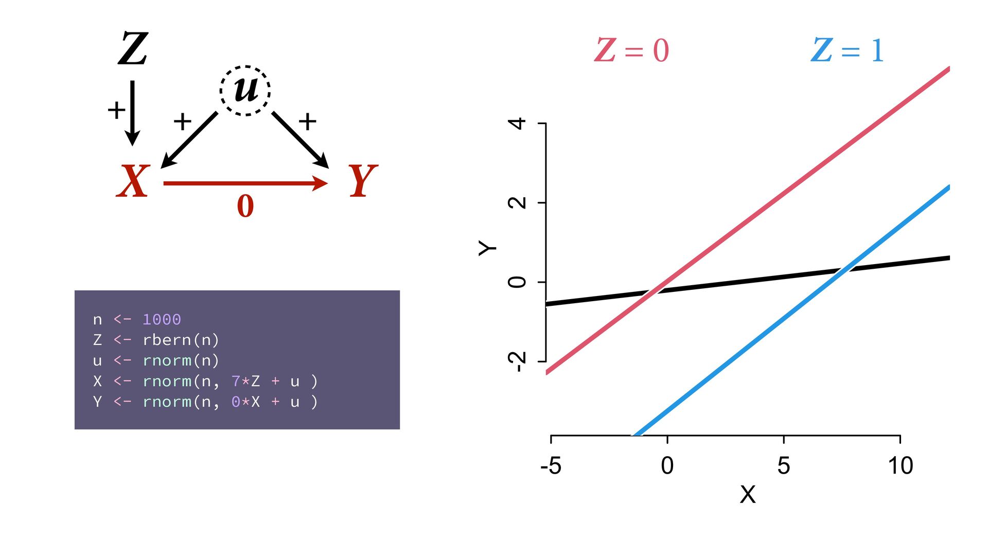
86. X Y Z u -0.5 0.0 0.5 1.0 0 1 2 3 4 5 posterior mean Density Y ~ X biased Y ~ X + Z more bias true value is zero WHY? Covariation X & Y requires variation in their causes Within each level of Z, less variation in X Confound u relatively more important within each Z
87. -5 0 5 10 -2 0 2 4 X Y X Y Z u 0 + + + n <- 1000 Z <- rbern(n) u <- rnorm(n) X <- rnorm(n, 7*Z + u ) Y <- rnorm(n, 0*X + u ) Z = 0 Z = 1
88. Good & Bad Controls “Control” variable: Variable introduced to an analysis so that a causal estimate is possible Heuristics fail — adding control variables can be worse than omitting Make assumptions explicit MODEL
 ALL THE THINGS
89. PAUSE
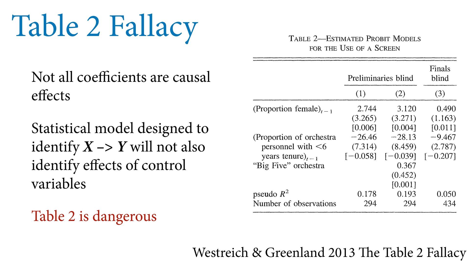
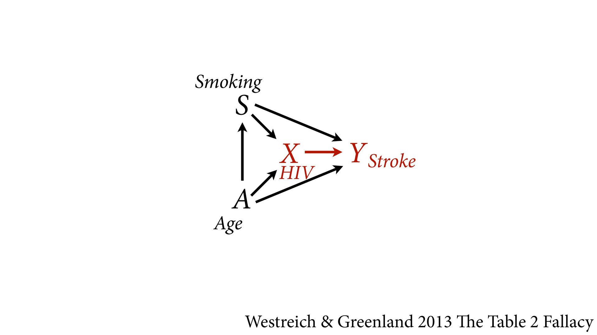
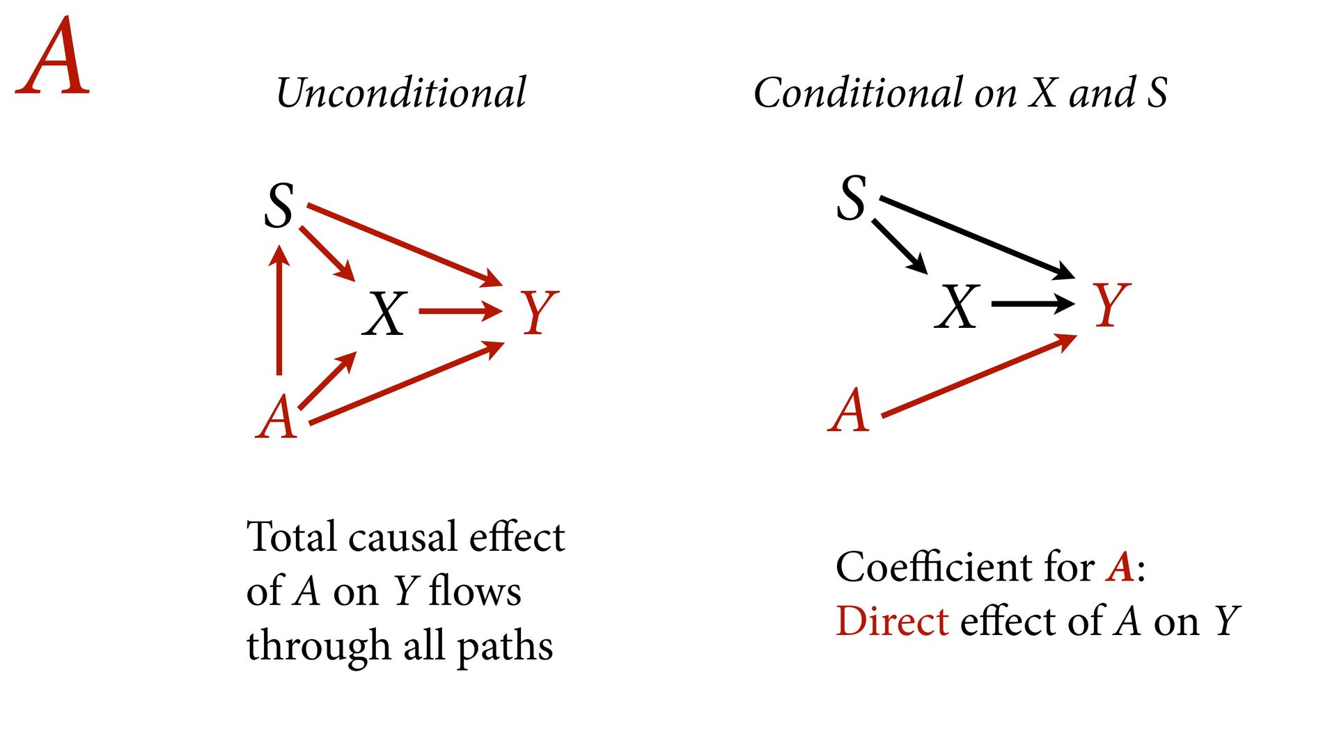
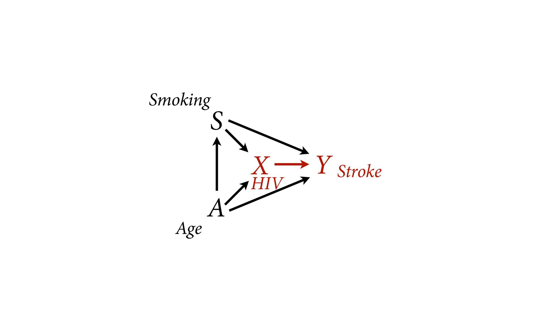
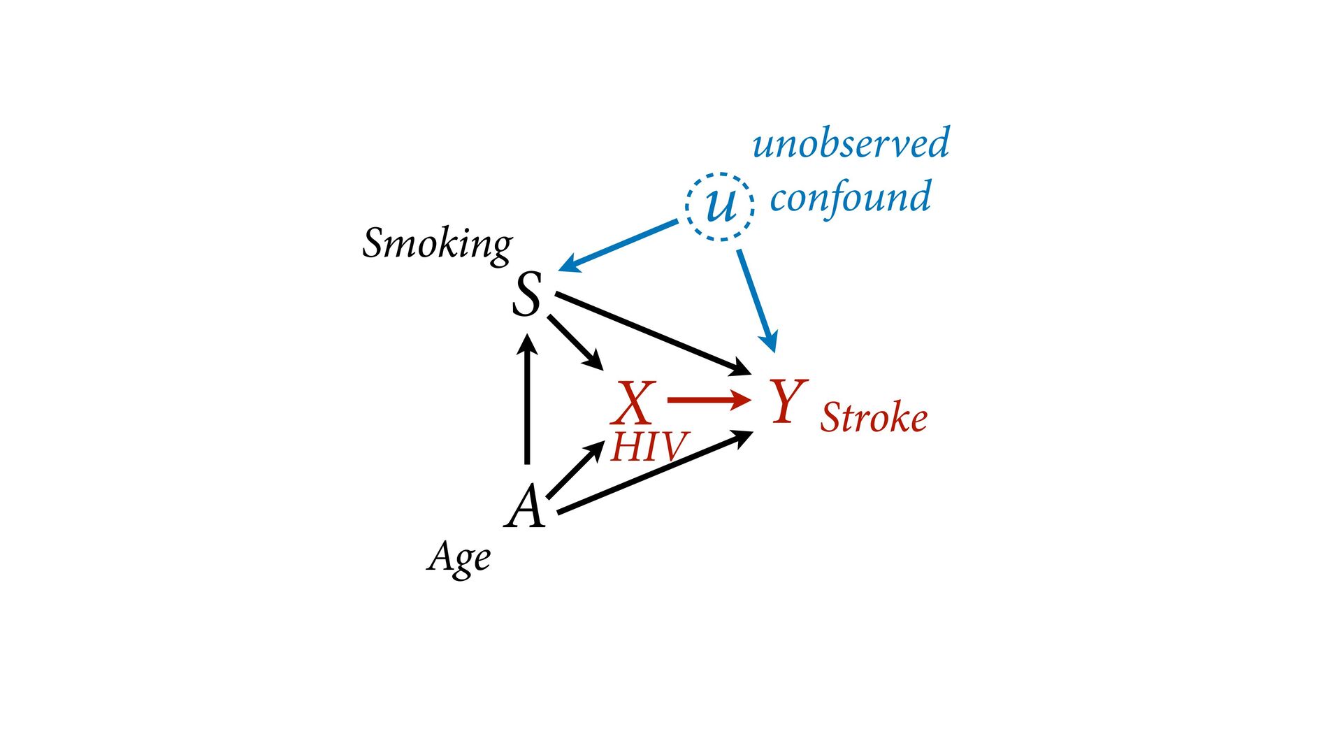
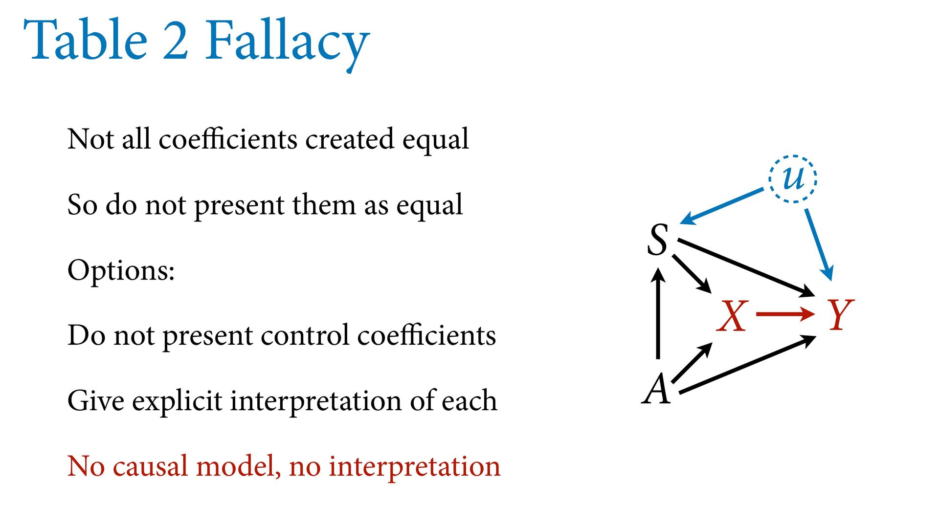
90. Table 2 Fallacy Not all coefficients are causal effects Statistical model designed to identify X –> Y will not also identify effects of control variables Table 2 is dangerous Westreich & Greenland 2013 The Table 2 Fallacy 724 THE AMERICAN EC TABLE 2-ESTIMATED PROBIT MODELS FOR THE USE OF A SCREEN Finals Preliminaries blind blind (1) (2) (3) (Proportion female),_ 2.744 3.120 0.490 (3.265) (3.271) (1.163) [0.006] [0.004] [0.011] (Proportion of orchestra -26.46 -28.13 -9.467 personnel with <6 (7.314) (8.459) (2.787) years tenure),- 1 [-0.058] [-0.039] [-0.207] "Big Five" orchestra 0.367 (0.452) [0.001] pseudo R2 0.178 0.193 0.050 Number of observations 294 294 434 Notes: The dependent variable is 1 if the orchestra adopts a screen, 0 otherwise. Huber standard errors (with orchestra random effects) are in parentheses. All specifications in- clude a constant. Changes in probabilities are in brackets.
91. A X Y S Westreich & Greenland 2013 The Table 2 Fallacy Stroke HIV Smoking Age
93. Use Backdoor Criterion A X Y S
94. Use Backdoor Criterion A X Y S X Y
95. Use Backdoor Criterion A X Y S X Y X Y S
96. Use Backdoor Criterion A X Y S X Y X Y S A X Y
97. Use Backdoor Criterion A X Y S X Y X Y S A X Y A X Y S
98. Use Backdoor Criterion A X Y S X Y X Y S A X Y A X Y S
99. Y i ∼ Normal(μ i , σ) μ i = α + β X X i + β S S i + β A A i A X Y S
100. A X Y S Confounded by A and S Unconditional X
101. Coefficient for X: 
 Effect of X on Y (still must marginalize!) A X Y S Confounded by A and S A X Y S Unconditional Conditional on A and S X
102. A X Y S Effect of S confounded by A Unconditional S
103. Coefficient for S: 
 Direct effect of S on Y A X Y S Effect of S confounded by A Unconditional Conditional on A and X A X Y S S
104. A X Y S Total causal effect of A on Y flows through all paths Unconditional A
105. Coefficient for A: 
 Direct effect of A on Y A X Y S Total causal effect of A on Y flows through all paths Unconditional Conditional on X and S A X Y S A
106. A X Y S Stroke HIV Smoking Age
107. A X Y S Stroke HIV Smoking Age u unobserved confound
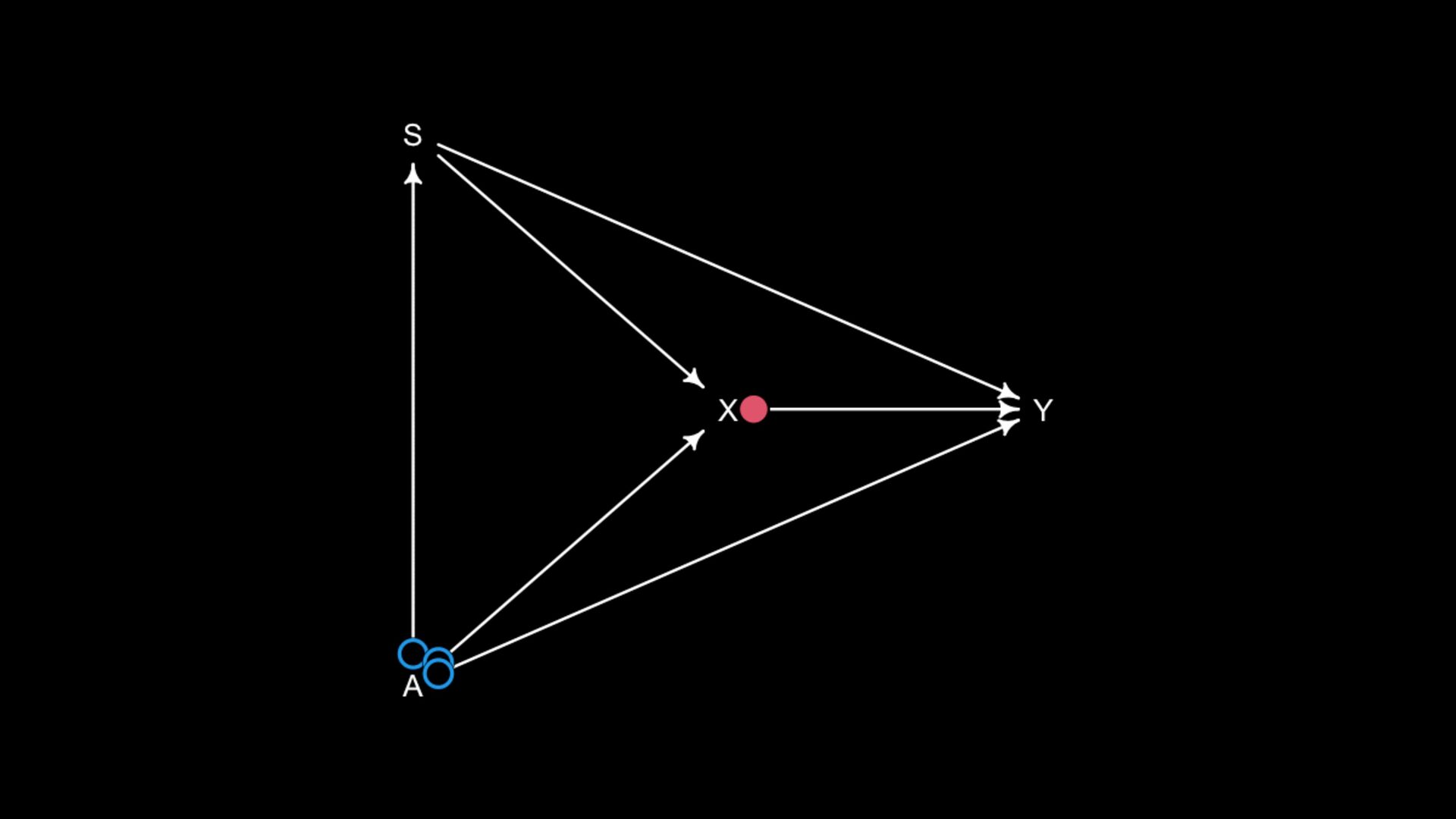
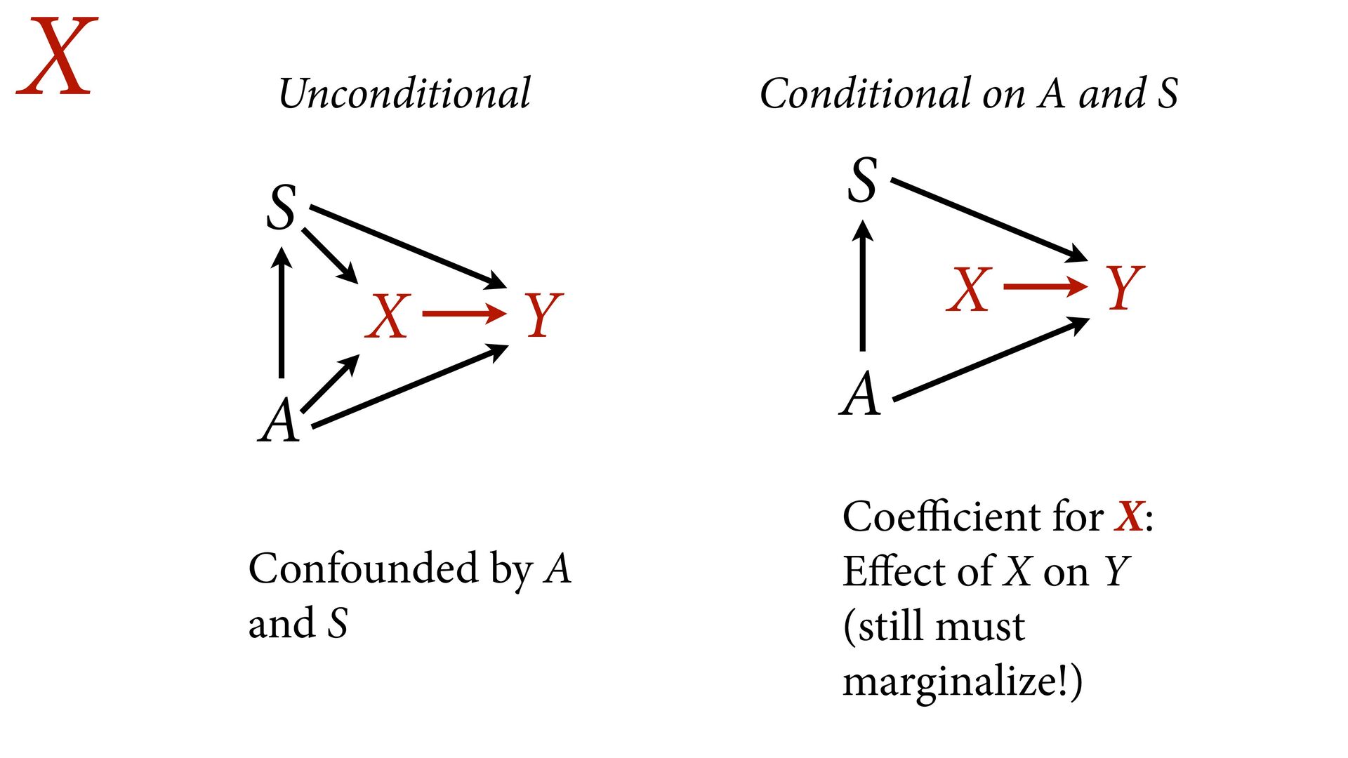
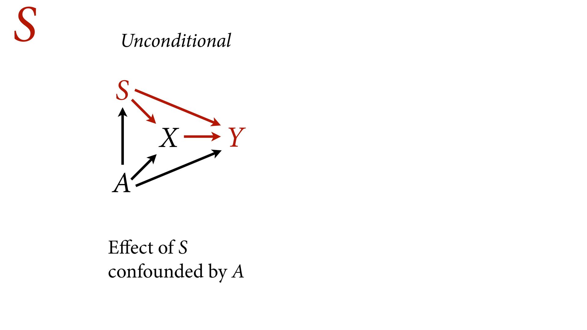
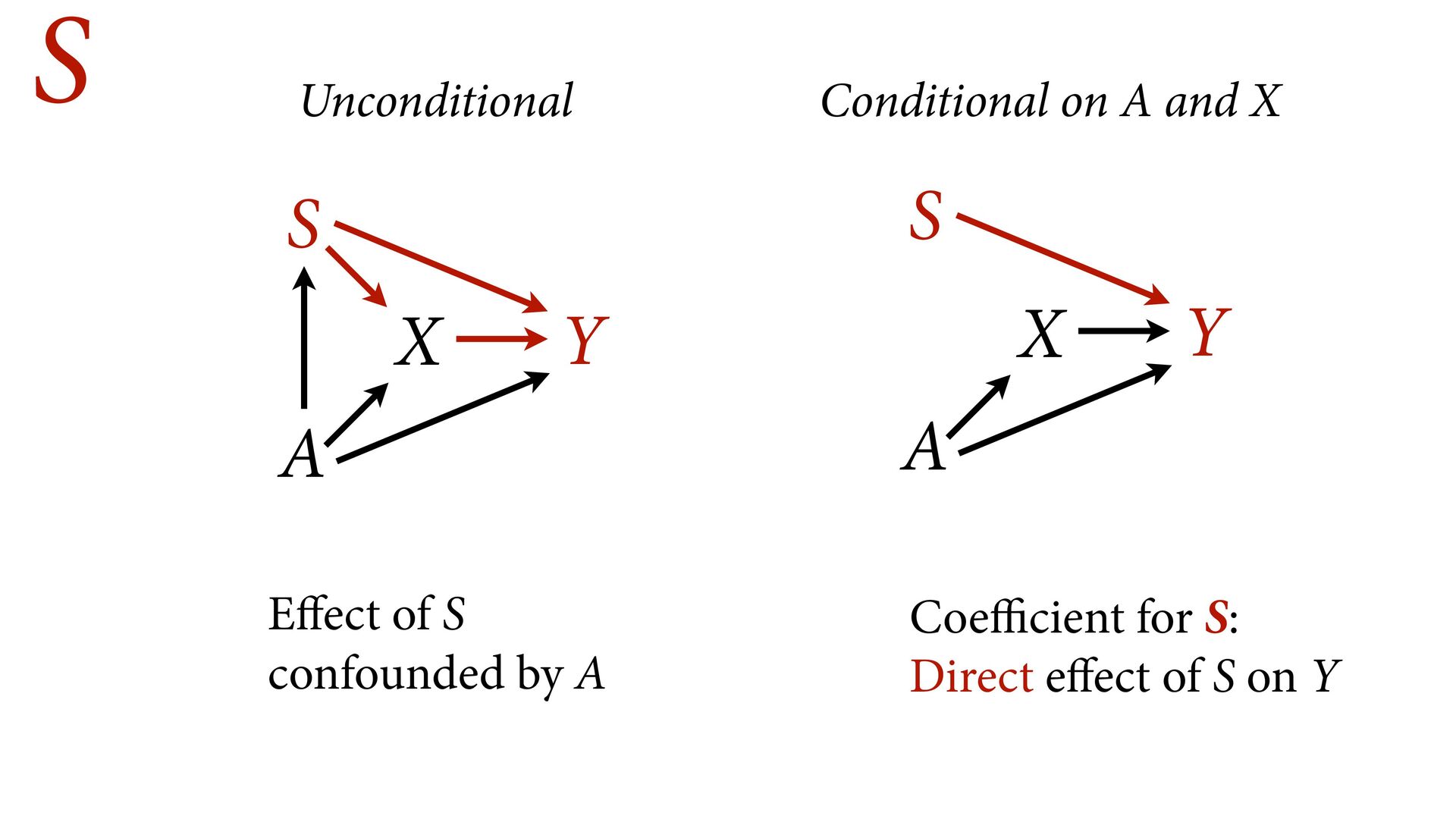
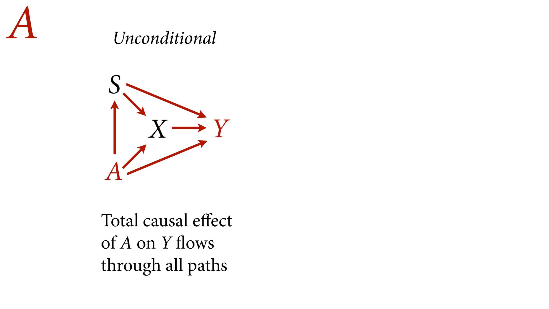
108. Table 2 Fallacy Not all coefficients created equal So do not present them as equal Options: Do not present control coefficients Give explicit interpretation of each No causal model, no interpretation A X Y S u
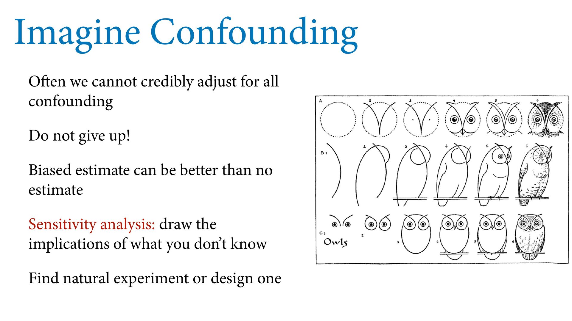
109. Imagine Confounding Often we cannot credibly adjust for all confounding Do not give up! Biased estimate can be better than no estimate Sensitivity analysis: draw the implications of what you don’t know Find natural experiment or design one
110. Course Schedule Week 1 Bayesian inference Chapters 1, 2, 3 Week 2 Linear models & Causal Inference Chapter 4 Week 3 Causes, Confounds & Colliders Chapters 5 & 6 Week 4 Overfitting / MCMC Chapters 7, 8, 9 Week 5 Generalized Linear Models Chapters 10, 11 Week 6 Integers & Other Monsters Chapters 11 & 12 Week 7 Multilevel models I Chapter 13 Week 8 Multilevel models II Chapter 14 Week 9 Measurement & Missingness Chapter 15 Week 10 Generalized Linear Madness Chapter 16 https://github.com/rmcelreath/stat_rethinking_2022