Statistical Rethinking 2022 Lecture 10

Course materials: https://github.com/rmcelreath/stat_rethinking_2022

Transcript

1. Statistical Rethinking 10: Counts and Confounds 2022
4. Generalized Linear Models Linear Models: Expected value is additive (“linear”) combination of parameters Generalized Linear Models: Expected value is some function of an additive combination of parameters Y i ∼ Normal(μ i , σ) μ i = α + β X X i + β Z Z i Y i ∼ Bernoulli(p i ) f(p i ) = α + β X X i + β Z Z i f(p i )
5. logit(p i ) = α + βx i Generalized Linear Models: Expected value is some function of an additive combination of parameters Uniform changes in predictor not uniform changes in prediction All predictor variables interact, moderate one another Influences predictions & uncertainty of predictions
6. Confounded Admissions G D A gender department admission
7. Confounded Admissions G D A gender department admission uability
8. set.seed(17) N <- 2000 # number of applicants # even gender distribution G <- sample( 1:2 , size=N , replace=TRUE ) # sample ability, high (1) to average (0) u <- rbern(N,0.1) # gender 1 tends to apply to department 1, 2 to 2 # and G=1 with greater ability tend to apply to 2 as well D <- rbern( N , ifelse( G==1 , u*0.5 , 0.8 ) ) + 1 # matrix of acceptance rates [dept,gender] accept_rate_u0 <- matrix( c(0.1,0.1,0.1,0.3) , nrow=2 ) accept_rate_u1 <- matrix( c(0.2,0.3,0.2,0.5) , nrow=2 ) # simulate acceptance p <- sapply( 1:N , function(i) ifelse( u[i]==0 , accept_rate_u0[D[i],G[i]] , accept_rate_u1[D[i],G[i]] ) ) A <- rbern( N , p ) G D A u
9. set.seed(17) N <- 2000 # number of applicants # even gender distribution G <- sample( 1:2 , size=N , replace=TRUE ) # sample ability, high (1) to average (0) u <- rbern(N,0.1) # gender 1 tends to apply to department 1, 2 to 2 # and G=1 with greater ability tend to apply to 2 as well D <- rbern( N , ifelse( G==1 , u*0.5 , 0.8 ) ) + 1 # matrix of acceptance rates [dept,gender] accept_rate_u0 <- matrix( c(0.1,0.1,0.1,0.3) , nrow=2 ) accept_rate_u1 <- matrix( c(0.2,0.3,0.2,0.5) , nrow=2 ) # simulate acceptance p <- sapply( 1:N , function(i) ifelse( u[i]==0 , accept_rate_u0[D[i],G[i]] , accept_rate_u1[D[i],G[i]] ) ) A <- rbern( N , p ) G D A u
10. set.seed(17) N <- 2000 # number of applicants # even gender distribution G <- sample( 1:2 , size=N , replace=TRUE ) # sample ability, high (1) to average (0) u <- rbern(N,0.1) # gender 1 tends to apply to department 1, 2 to 2 # and G=1 with greater ability tend to apply to 2 as well D <- rbern( N , ifelse( G==1 , u*0.5 , 0.8 ) ) + 1 # matrix of acceptance rates [dept,gender] accept_rate_u0 <- matrix( c(0.1,0.1,0.1,0.3) , nrow=2 ) accept_rate_u1 <- matrix( c(0.2,0.3,0.2,0.5) , nrow=2 ) # simulate acceptance p <- sapply( 1:N , function(i) ifelse( u[i]==0 , accept_rate_u0[D[i],G[i]] , accept_rate_u1[D[i],G[i]] ) ) A <- rbern( N , p ) G D A u
11. set.seed(17) N <- 2000 # number of applicants # even gender distribution G <- sample( 1:2 , size=N , replace=TRUE ) # sample ability, high (1) to average (0) u <- rbern(N,0.1) # gender 1 tends to apply to department 1, 2 to 2 # and G=1 with greater ability tend to apply to 2 as well D <- rbern( N , ifelse( G==1 , u*0.5 , 0.8 ) ) + 1 # matrix of acceptance rates [dept,gender] accept_rate_u0 <- matrix( c(0.1,0.1,0.1,0.3) , nrow=2 ) accept_rate_u1 <- matrix( c(0.2,0.3,0.2,0.5) , nrow=2 ) # simulate acceptance p <- sapply( 1:N , function(i) ifelse( u[i]==0 , accept_rate_u0[D[i],G[i]] , accept_rate_u1[D[i],G[i]] ) ) A <- rbern( N , p ) G D A u
12. set.seed(17) N <- 2000 # number of applicants # even gender distribution G <- sample( 1:2 , size=N , replace=TRUE ) # sample ability, high (1) to average (0) u <- rbern(N,0.1) # gender 1 tends to apply to department 1, 2 to 2 # and G=1 with greater ability tend to apply to 2 as well D <- rbern( N , ifelse( G==1 , u*0.5 , 0.8 ) ) + 1 # matrix of acceptance rates [dept,gender] accept_rate_u0 <- matrix( c(0.1,0.1,0.1,0.3) , nrow=2 ) accept_rate_u1 <- matrix( c(0.2,0.3,0.2,0.5) , nrow=2 ) # simulate acceptance p <- sapply( 1:N , function(i) ifelse( u[i]==0 , accept_rate_u0[D[i],G[i]] , accept_rate_u1[D[i],G[i]] ) ) A <- rbern( N , p ) G D A u > accept_rate_u0 [,1] [,2] [1,] 0.1 0.1 [2,] 0.1 0.3 > accept_rate_u1 [,1] [,2] [1,] 0.2 0.2 [2,] 0.3 0.5
13. dat_sim <- list( A=A , D=D , G=G ) # total effect gender m1 <- ulam( alist( A ~ bernoulli(p), logit(p) <- a[G], a[G] ~ normal(0,1) ), data=dat_sim , chains=4 , cores=4 ) # direct effects - now confounded! m2 <- ulam( alist( A ~ bernoulli(p), logit(p) <- a[G,D], matrix[G,D]:a ~ normal(0,1) ), data=dat_sim , chains=4 , cores=4 ) > precis(m1,depth=2) mean sd 5.5% 94.5% n_eff Rhat4 a[1] -2.10 0.10 -2.26 -1.93 1297 1 a[2] -0.86 0.07 -0.97 -0.76 1008 1 > precis(m2,depth=3) mean sd 5.5% 94.5% n_eff Rhat4 a[1,1] -2.18 0.11 -2.35 -2.01 2083 1 a[1,2] -0.99 0.30 -1.49 -0.51 2408 1 a[2,1] -1.97 0.21 -2.31 -1.65 2335 1 a[2,2] -0.65 0.07 -0.77 -0.53 2260 1 Let’s look at the contrasts… total effect shows disadvantage direct effect confounded
14. -1.0 -0.5 0.0 0.5 1.0 0.0 0.5 1.0 1.5 F-M contrast in each department Density post2 <- extract.samples(m2) post2$fm_contrast_D1 <- post2$a[,1,1] - post2$a[,2,1] post2$fm_contrast_D2 <- post2$a[,1,2] - post2$a[,2,2] Dept 1 Dept 2 How can the confound hide discrimination?
15. You guessed it: Collider bias Stratifying by D opens non-causal path through u Can estimate total causal effect of G, but this isn’t what we want Cannot estimate direct effect of D or G G D A u
16. You guessed it: Collider bias More intuitive explanation: High ability G1s apply to discriminatory department anyway G1s in that department are higher ability on average than G2s High ability compensates for discrimination => masks evidence G D A u
17. Policing confounds X Z Y ethnicity stopped by police assaulted by police Knox Lowe & Mummolo 2020 Administrative Records Mask Racially Biased Policing
18. Policing confounds X Z Y ethnicity stopped by police assaulted by police uacting suspicious Data on police stops are confounded by lack of data on who wasn’t stopped: forced conditioning on Z Knox Lowe & Mummolo 2020 Administrative Records Mask Racially Biased Policing
19. # if we could measure u dat_sim$u <- u m3 <- ulam( alist( A ~ bernoulli(p), logit(p) <- a[G,D] + buA*u, matrix[G,D]:a ~ normal(0,1), buA ~ normal(0,1) ), data=dat_sim , constraints=list(buA="lower=0") , chains=4 , cores=4 ) post3 <- extract.samples(m3) post3$fm_contrast_D1 <- post3$a[,1,1] - post3$a[,2,1] post3$fm_contrast_D2 <- post3$a[,1,2] - post3$a[,2,2] Imagine we could measure the confound G D A u Need to block non-causal path through u
20. # if we could measure u dat_sim$u <- u m3 <- ulam( alist( A ~ bernoulli(p), logit(p) <- a[G,D] + buA*u, matrix[G,D]:a ~ normal(0,1), buA ~ normal(0,1) ), data=dat_sim , constraints=list(buA="lower=0") , chains=4 , cores=4 ) post3 <- extract.samples(m3) post3$fm_contrast_D1 <- post3$a[,1,1] - post3$a[,2,1] post3$fm_contrast_D2 <- post3$a[,1,2] - post3$a[,2,2] Imagine we could measure the confound Add u to linear model
21. # if we could measure u dat_sim$u <- u m3 <- ulam( alist( A ~ bernoulli(p), logit(p) <- a[G,D] + buA*u, matrix[G,D]:a ~ normal(0,1), buA ~ normal(0,1) ), data=dat_sim , constraints=list(buA="lower=0") , chains=4 , cores=4 ) post3 <- extract.samples(m3) post3$fm_contrast_D1 <- post3$a[,1,1] - post3$a[,2,1] post3$fm_contrast_D2 <- post3$a[,1,2] - post3$a[,2,2] Imagine we could measure the confound Constrain effect of u to +
22. # if we could measure u dat_sim$u <- u m3 <- ulam( alist( A ~ bernoulli(p), logit(p) <- a[G,D] + buA*u, matrix[G,D]:a ~ normal(0,1), buA ~ normal(0,1) ), data=dat_sim , constraints=list(buA="lower=0") , chains=4 , cores=4 ) post3 <- extract.samples(m3) post3$fm_contrast_D1 <- post3$a[,1,1] - post3$a[,2,1] post3$fm_contrast_D2 <- post3$a[,1,2] - post3$a[,2,2] Imagine we could measure the confound -2.0 -1.5 -1.0 -0.5 0.0 0.5 1.0 0.0 0.5 1.0 1.5 F-M contrast in each department Density Dept 1 Dept 2
23. De-confounding What can be done? Experiments Sensitivity analysis Measure proxies of confound G D A u
24. Sensitivity analysis What are the implications of what we don’t know? Assume confound exists, model its consequences for different strengths/kinds of influence How strong must the confound be to change conclusions? G D A u
25. Sensitivity analysis A i ∼ Bernoulli(p i ) logit(p i ) = α[G i , D i ] + β G[i] u i G D A u
26. Sensitivity analysis A i ∼ Bernoulli(p i ) logit(p i ) = α[G i , D i ] + β G[i] u i G D A u (D i = 2) ∼ Bernoulli(q i ) logit(q i ) = δ[G i ] + γ G[i] u i G D A u
27. A i ∼ Bernoulli(p i ) logit(p i ) = α[G i , D i ] + β G[i] u i (D i = 2) ∼ Bernoulli(q i ) logit(q i ) = δ[G i ] + γ G[i] u i datl$D1 <- ifelse(datl$D==1,1,0) datl$N <- length(datl$D) datl$b <- c(1,1) datl$g <- c(1,0) mGDu <- ulam( alist( # A model A ~ bernoulli(p), logit(p) <- a[G,D] + b[G]*u[i], matrix[G,D]:a ~ normal(0,1), # D model D1 ~ bernoulli(q), logit(q) <- delta[G] + g[G]*u[i], delta[G] ~ normal(0,1), # declare unobserved u vector[N]:u ~ normal(0,1) ), data=datl , chains=4 , cores=4 ) u j ∼ Normal(0,1)
28. datl$D1 <- ifelse(datl$D==1,1,0) datl$N <- length(datl$D) datl$b <- c(1,1) datl$g <- c(1,0) mGDu <- ulam( alist( # A model A ~ bernoulli(p), logit(p) <- a[G,D] + b[G]*u[i], matrix[G,D]:a ~ normal(0,1), # D model D1 ~ bernoulli(q), logit(q) <- delta[G] + g[G]*u[i], delta[G] ~ normal(0,1), # declare unobserved u vector[N]:u ~ normal(0,1) ), data=datl , chains=4 , cores=4 ) -1.0 -0.5 0.0 0.5 1.0 1.5 0.0 0.5 1.0 1.5 F-M contrast in department A Density
29. 0 200 400 600 800 -1.0 0.0 0.5 1.0 1.5 application to department A posterior u men rejected women
 rejected men admitted women
 admitted Posterior u values, Department A
30. Sensitivity analysis What are the implications of what we don’t know? Somewhere between pure simulation and pure analysis Vary confound strength over range and show how results change –or– vary other effects and estimate confound strength Confounds often persist — don’t pretend G D A u -1.0 -0.5 0.0 0.5 1.0 1.5 0.0 0.5 1.0 1.5 F-M contrast in department A Density assuming
 confounds ignoring
 confounds
31. De-confounding G D A gender department admission u T1 T2 test score test score
32. A i ∼ Bernoulli(p i ) logit(p i ) = α[G i , D i ] + β G[i] u i T i,j ∼ Normal(u i , τ j ) u k ∼ Normal(0,1) De-confounding G D A u T1,2,3 G D A u T1,2,3
33. T1 <- rnorm(N,u,0.1) T2 <- rnorm(N,u,0.5) T3 <- rnorm(N,u,0.25) m4 <- ulam( alist( # A model A ~ bernoulli(p), logit(p) <- a[G,D] + b*u[i], matrix[G,D]:a ~ normal(0,1), b ~ normal(0,1), # u and T model vector[N]:u ~ normal(0,1), T1 ~ normal(u,tau[1]), T2 ~ normal(u,tau[2]), T3 ~ normal(u,tau[3]), vector[3]:tau ~ exponential(1) ), data=dat_sim , chains=4 , cores=4 , constraints=list(b="lower=0") ) A i ∼ Bernoulli(p i ) logit(p i ) = α[G i , D i ] + β G[i] u i T i,j ∼ Normal(u i , τ j ) u k ∼ Normal(0,1) *This model samples inefficiently; learn to fix later in course
34. 0.0 0.5 1.0 u (true) posterior mean u 0 1 inferring
 confound ignoring
 confound -2.0 -1.5 -1.0 -0.5 0.0 0.5 1.0 0.0 0.5 1.0 1.5 F-M contrast in each department Density u k ∼ Normal(0,1)
35. 0.0 0.5 1.0 u (true) posterior mean u 0 1 inferring
 confound ignoring
 confound -2.0 -1.5 -1.0 -0.5 0.0 0.5 1.0 0.0 0.5 1.0 1.5 F-M contrast in each department Density u k ∼ Normal(0,1) More parameters (2008) than observations (2000)!
36. Charlie Chaplin, Modern Times (1936)
37. PAUSE
38. Oceanic tool complexity How is technological complexity related to population size? To social structure? data(Kline) culture population contact total_tools mean_TU 1 Malekula 1100 low 13 3.2 2 Tikopia 1500 low 22 4.7 3 Santa Cruz 3600 low 24 4.0 4 Yap 4791 high 43 5.0 5 Lau Fiji 7400 high 33 5.0 6 Trobriand 8000 high 19 4.0 7 Chuuk 9200 high 40 3.8 8 Manus 13000 low 28 6.6 9 Tonga 17500 high 55 5.4 10 Hawaii 275000 low 71 6.6 Estimand: Causal influence of population size and contact on total tools Kline & Boyd 2010 Population size predicts technological complexity in Oceania
39. Technological complexity Tools Innovations Population Loss Contact
40. Technological complexity P C T L contact population tools location
41. Technological complexity P C T L contact population tools location Adjustment set for P: L Also want to stratify by C, to study interaction
42. Modeling tools Tool count is not binomial: No maximum Poisson distribution: Very high maximum and very low probability of each success Here: Many many possible technologies, very few realized in any one place
43. Poisson link is log Poisson distribution takes shape from expected value Must be positive Exponential scaling can be surprising! Y i ∼ Poisson(λ i ) log(λ i ) = α + βx i λ i = exp(α + βx i ) log(λ i ) exp
44. Poisson (poison) priors Exponential scaling can be surprising α ∼ Normal(0,10) log(λ i ) = α
45. Poisson (poison) priors Exponential scaling can be surprising α ∼ Normal(0,10) log(λ i ) = α 0 20 40 60 80 100 0.00 0.01 0.02 0.03 0.04 0.05 mean number of tools Density
46. 0 20 40 60 80 100 0.00 0.01 0.02 0.03 0.04 0.05 mean number of tools Density Poisson (poison) priors Exponential scaling can be surprising α ∼ Normal(0,10) log(λ i ) = α α ∼ Normal(3,0.5)
47. Poisson priors -2 -1 0 1 2 0 20 40 60 80 100 x value expected count α ∼ Normal(0,1) log(λ i ) = α + βx i β ∼ Normal(0,10) -2 -1 0 1 2 0 20 40 60 80 100 x value expected count α ∼ Normal(3,0.5) β ∼ Normal(0,0.2)
48. data(Kline) d <- Kline d$P <- scale( log(d$population) ) d$contact_id <- ifelse( d$contact=="high" , 2 , 1 ) dat <- list( T = d$total_tools , P = d$P , C = d$contact_id ) # intercept only m11.9 <- ulam( alist( T ~ dpois( lambda ), log(lambda) <- a, a ~ dnorm( 3 , 0.5 ) ), data=dat , chains=4 , log_lik=TRUE ) # interaction model m11.10 <- ulam( alist( T ~ dpois( lambda ), log(lambda) <- a[C] + b[C]*P, a[C] ~ dnorm( 3 , 0.5 ), b[C] ~ dnorm( 0 , 0.2 ) ), data=dat , chains=4 , log_lik=TRUE ) compare( m11.9 , m11.10 , func=PSIS ) Y i ∼ Poisson(λ i ) log(λ i ) = α C[i] + β C[i] log(P i ) α j ∼ Normal(3,0.5) β j ∼ Normal(0,0.2)
49. data(Kline) d <- Kline d$P <- scale( log(d$population) ) d$contact_id <- ifelse( d$contact=="high" , 2 , 1 ) dat <- list( T = d$total_tools , P = d$P , C = d$contact_id ) # intercept only m11.9 <- ulam( alist( T ~ dpois( lambda ), log(lambda) <- a, a ~ dnorm( 3 , 0.5 ) ), data=dat , chains=4 , log_lik=TRUE ) # interaction model m11.10 <- ulam( alist( T ~ dpois( lambda ), log(lambda) <- a[C] + b[C]*P, a[C] ~ dnorm( 3 , 0.5 ), b[C] ~ dnorm( 0 , 0.2 ) ), data=dat , chains=4 , log_lik=TRUE ) compare( m11.9 , m11.10 , func=PSIS ) Y i ∼ Poisson(λ i ) log(λ i ) = α C[i] + β C[i] log(P i ) α j ∼ Normal(3,0.5) β j ∼ Normal(0,0.2) > compare( m11.9 , m11.10 , func=PSIS ) Some Pareto k values are high (>0.5). Set pointwise=TRUE to inspect individual points. Some Pareto k values are high (>0.5). Set pointwise=TRUE to inspect individual points. PSIS SE dPSIS dSE pPSIS weight m11.10 85.9 13.50 0.0 NA 7.3 1 m11.9 141.3 33.69 55.4 33.13 8.0 0
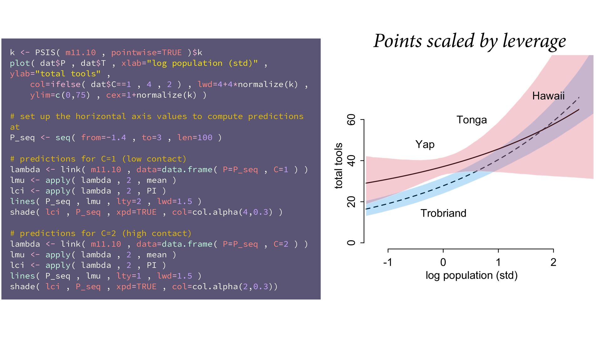
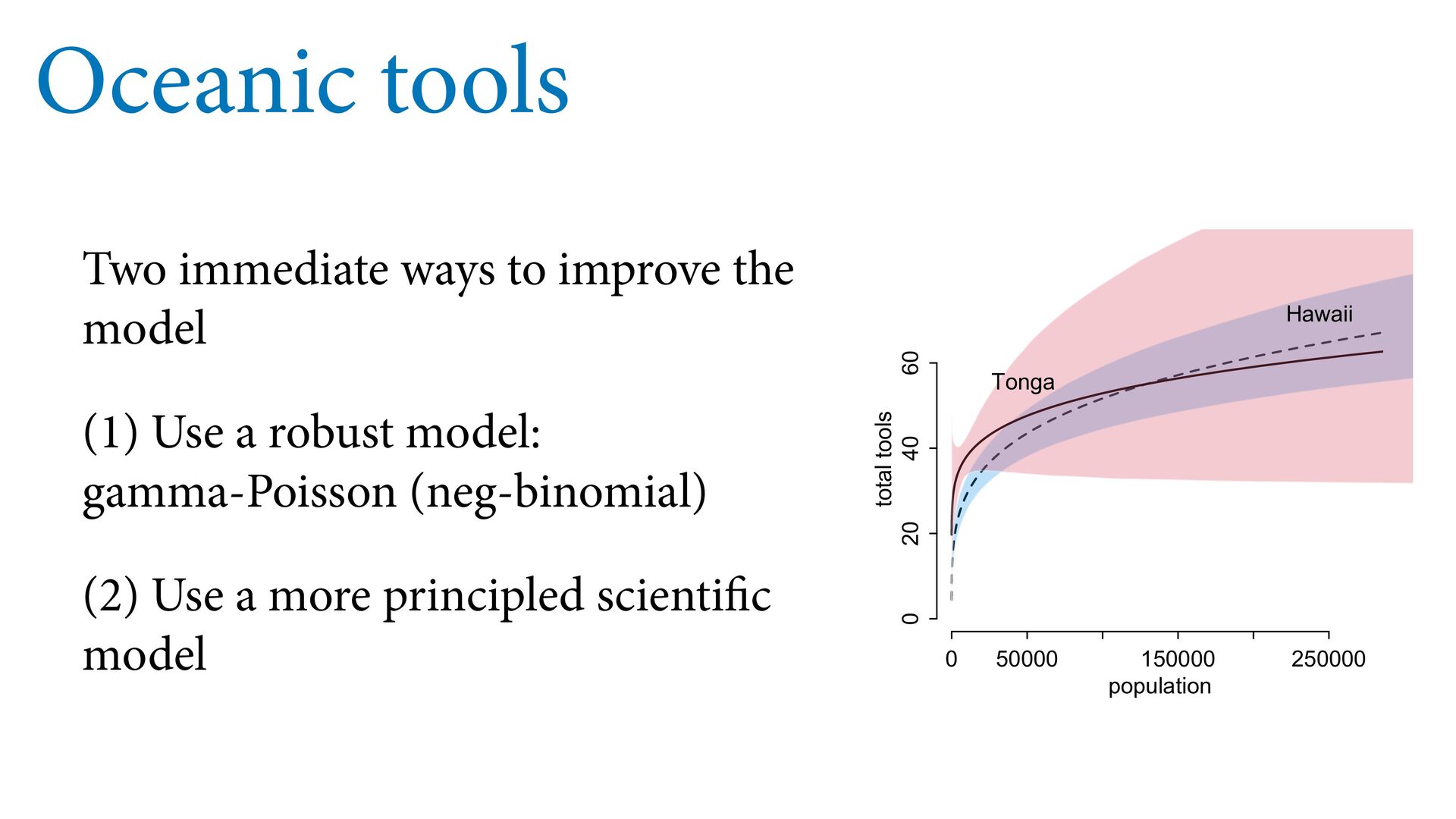
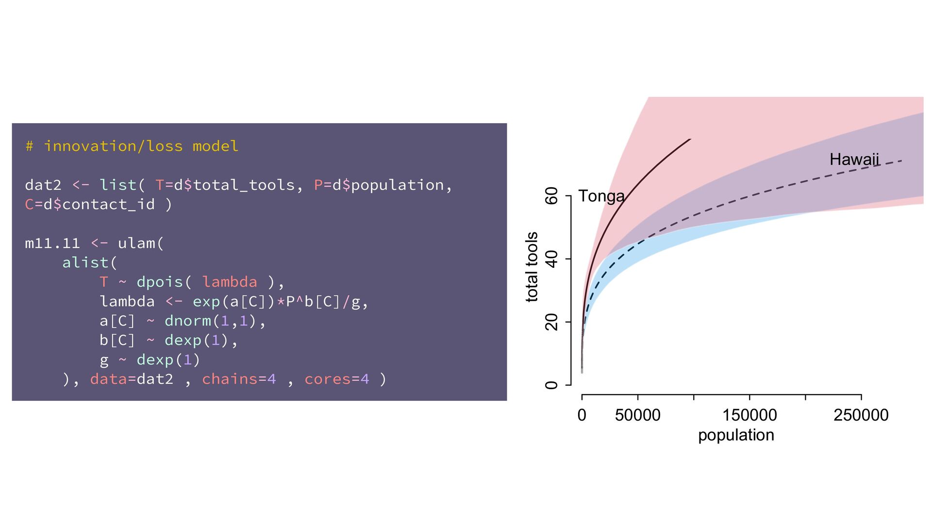
50. -1 0 1 2 0 20 40 60 log population (std) total tools Yap Trobriand Tonga Hawaii k <- PSIS( m11.10 , pointwise=TRUE )$k plot( dat$P , dat$T , xlab="log population (std)" , ylab="total tools" , col=ifelse( dat$C==1 , 4 , 2 ) , lwd=4+4*normalize(k) , ylim=c(0,75) , cex=1+normalize(k) ) # set up the horizontal axis values to compute predictions at P_seq <- seq( from=-1.4 , to=3 , len=100 ) # predictions for C=1 (low contact) lambda <- link( m11.10 , data=data.frame( P=P_seq , C=1 ) ) lmu <- apply( lambda , 2 , mean ) lci <- apply( lambda , 2 , PI ) lines( P_seq , lmu , lty=2 , lwd=1.5 ) shade( lci , P_seq , xpd=TRUE , col=col.alpha(4,0.3) ) # predictions for C=2 (high contact) lambda <- link( m11.10 , data=data.frame( P=P_seq , C=2 ) ) lmu <- apply( lambda , 2 , mean ) lci <- apply( lambda , 2 , PI ) lines( P_seq , lmu , lty=1 , lwd=1.5 ) shade( lci , P_seq , xpd=TRUE , col=col.alpha(2,0.3)) Points scaled by leverage
51. -1 0 1 2 0 20 40 60 log population (std) total tools Yap Trobriand Tonga Hawaii 0 50000 150000 250000 0 20 40 60 population total tools Tonga Hawaii log scale Natural scale
52. 0 50000 150000 250000 0 20 40 60 population total tools Tonga Hawaii
53. 0 50000 150000 250000 0 20 40 6 total tools Tonga
54. Oceanic tools Two immediate ways to improve the model (1) Use a robust model: 
 gamma-Poisson (neg-binomial) (2) Use a more principled scientific model 0 50000 150000 250000 0 20 40 60 population total tools Tonga Hawaii
55. Technological complexity
56. ΔT = αPβ − γT
57. ΔT = αPβ − γT change in tools innovation rate diminishing returns
 (elasticity) rate of loss
58. ΔT = α C Pβ C − γT diminishing returns
 depend upon contact innovation depends upon contact
59. ΔT = α C Pβ C − γT = 0 Solve for T
60. ΔT = α C Pβ C − γT = 0 Solve for T ̂ T = α C Pβ C γ
61. ̂ T = α C Pβ C γ T i ∼ Poisson(λ i ) λ i = ̂ T
62. # innovation/loss model dat2 <- list( T=d$total_tools, P=d$population, C=d$contact_id ) m11.11 <- ulam( alist( T ~ dpois( lambda ), lambda <- exp(a[C])*P^b[C]/g, a[C] ~ dnorm(1,1), b[C] ~ dexp(1), g ~ dexp(1) ), data=dat2 , chains=4 , cores=4 ) All parameters must be positive Two ways to do this (1) use exp() (2) use appropriate prior
63. # innovation/loss model dat2 <- list( T=d$total_tools, P=d$population, C=d$contact_id ) m11.11 <- ulam( alist( T ~ dpois( lambda ), lambda <- exp(a[C])*P^b[C]/g, a[C] ~ dnorm(1,1), b[C] ~ dexp(1), g ~ dexp(1) ), data=dat2 , chains=4 , cores=4 ) All parameters must be positive Two ways to do this (1) use exp() (2) use appropriate prior > precis(m11.11,2) mean sd 5.5% 94.5% n_eff Rhat4 a[1] 0.85 0.68 -0.26 1.90 698 1 a[2] 0.93 0.83 -0.39 2.31 902 1 b[1] 0.26 0.03 0.21 0.32 1149 1 b[2] 0.29 0.10 0.12 0.45 711 1 g 1.11 0.70 0.32 2.43 862 1
64. # innovation/loss model dat2 <- list( T=d$total_tools, P=d$population, C=d$contact_id ) m11.11 <- ulam( alist( T ~ dpois( lambda ), lambda <- exp(a[C])*P^b[C]/g, a[C] ~ dnorm(1,1), b[C] ~ dexp(1), g ~ dexp(1) ), data=dat2 , chains=4 , cores=4 ) 0 50000 150000 250000 0 20 40 60 population total tools Tonga Hawaii
65. 0 50000 150000 250000 0 20 40 60 population total tools Tonga Hawaii 0 50000 150000 250000 0 20 40 60 population total tools Tonga Hawaii Innovation/loss model Generalized linear model Still have to deal with location as confound
66. Count GLMs Before you see the values, you know a count is zero or positive Maximum entropy priors: Binomial, Poisson, and extensions More event types: Multinomial and categorical Robust regressions: 
 Beta-binomial, gamma-Poisson (neg-binomial) Examples to come
67. Course Schedule Week 1 Bayesian inference Chapters 1, 2, 3 Week 2 Linear models & Causal Inference Chapter 4 Week 3 Causes, Confounds & Colliders Chapters 5 & 6 Week 4 Overfitting / MCMC Chapters 7, 8, 9 Week 5 Generalized Linear Models Chapters 10, 11 Week 6 Mixtures & ordered categories Chapters 11 & 12 Week 7 Multilevel models I Chapter 13 Week 8 Multilevel models II Chapter 14 Week 9 Measurement & Missingness Chapter 15 Week 10 Generalized Linear Madness Chapter 16 https://github.com/rmcelreath/stat_rethinking_2022