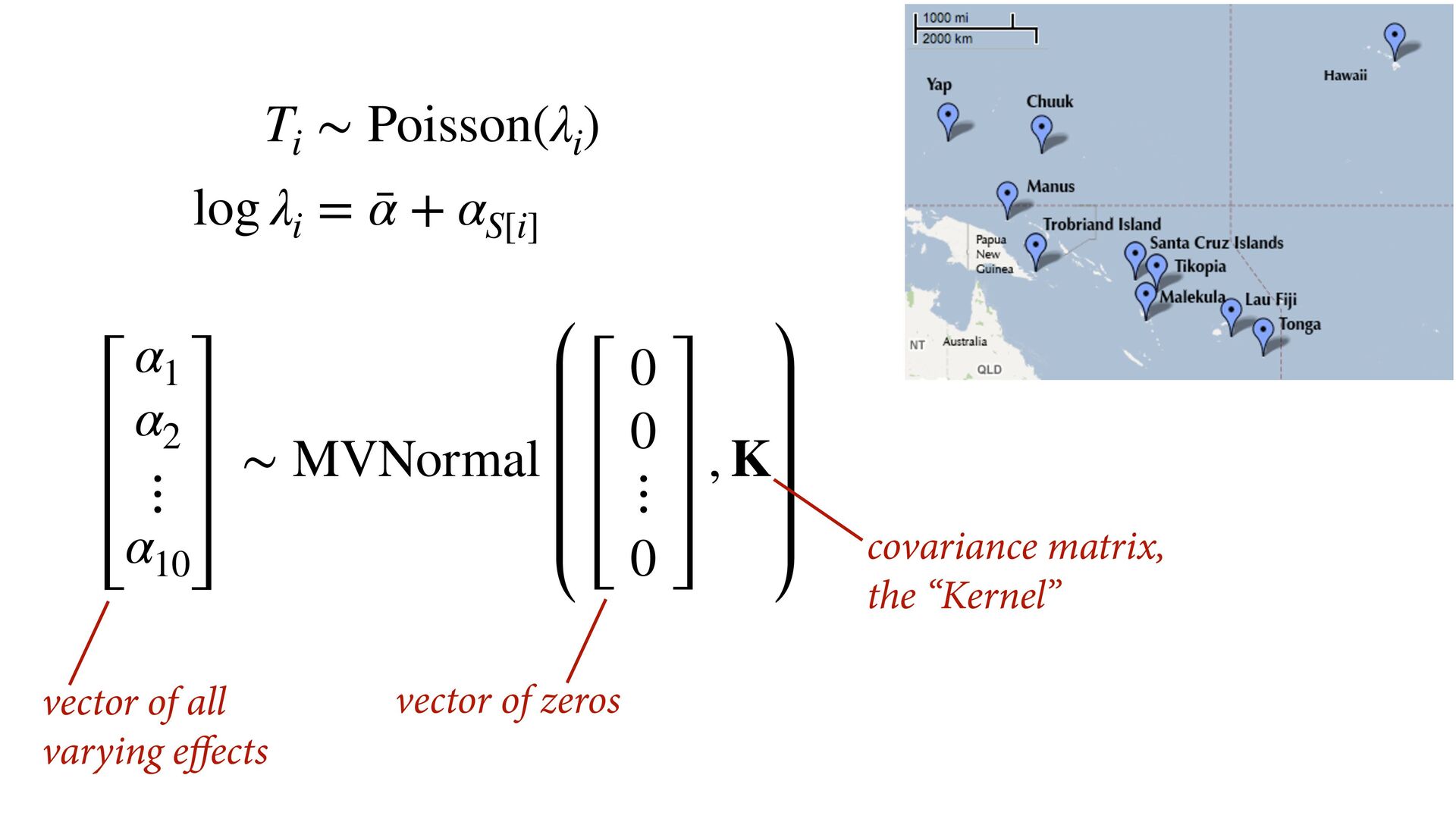
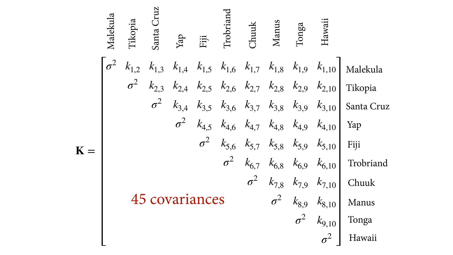
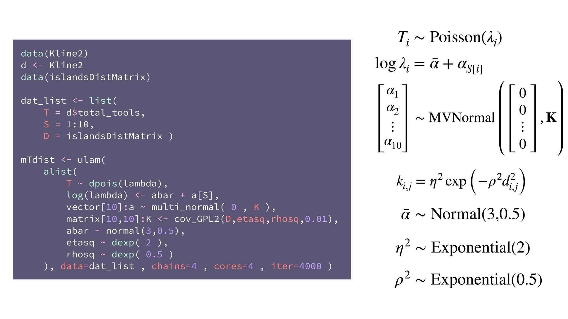
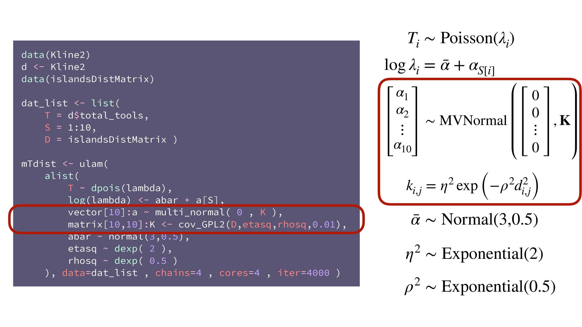
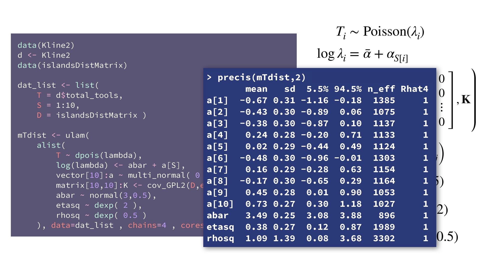
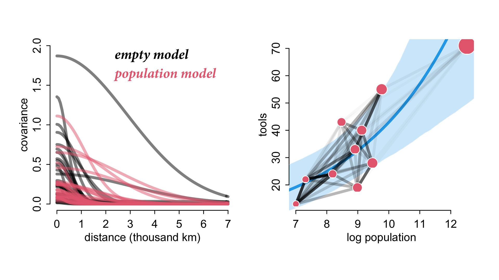
i ∼ Poisson(λ i ) α 1 α 2 ⋮ α 10 ∼ MVNormal 0 0 ⋮ 0 , K K = σ2 k 1,2 k 1,3 k 1,4 k 1,5 k 1,6 k 1,7 k 1,8 k 1,9 k 1,10 σ2 k 2,3 k 2,4 k 2,5 k 2,6 k 2,7 k 2,8 k 2,9 k 2,10 σ2 k 3,4 k 3,5 k 3,6 k 3,7 k 3,8 k 3,9 k 3,10 σ2 k 4,5 k 4,6 k 4,7 k 4,8 k 4,9 k 4,10 σ2 k 5,6 k 5,7 k 5,8 k 5,9 k 5,10 σ2 k 6,7 k 6,8 k 6,9 k 6,10 σ2 k 7,8 k 7,9 k 7,10 σ2 k 8,9 k 8,10 σ2 k 9,10 σ2
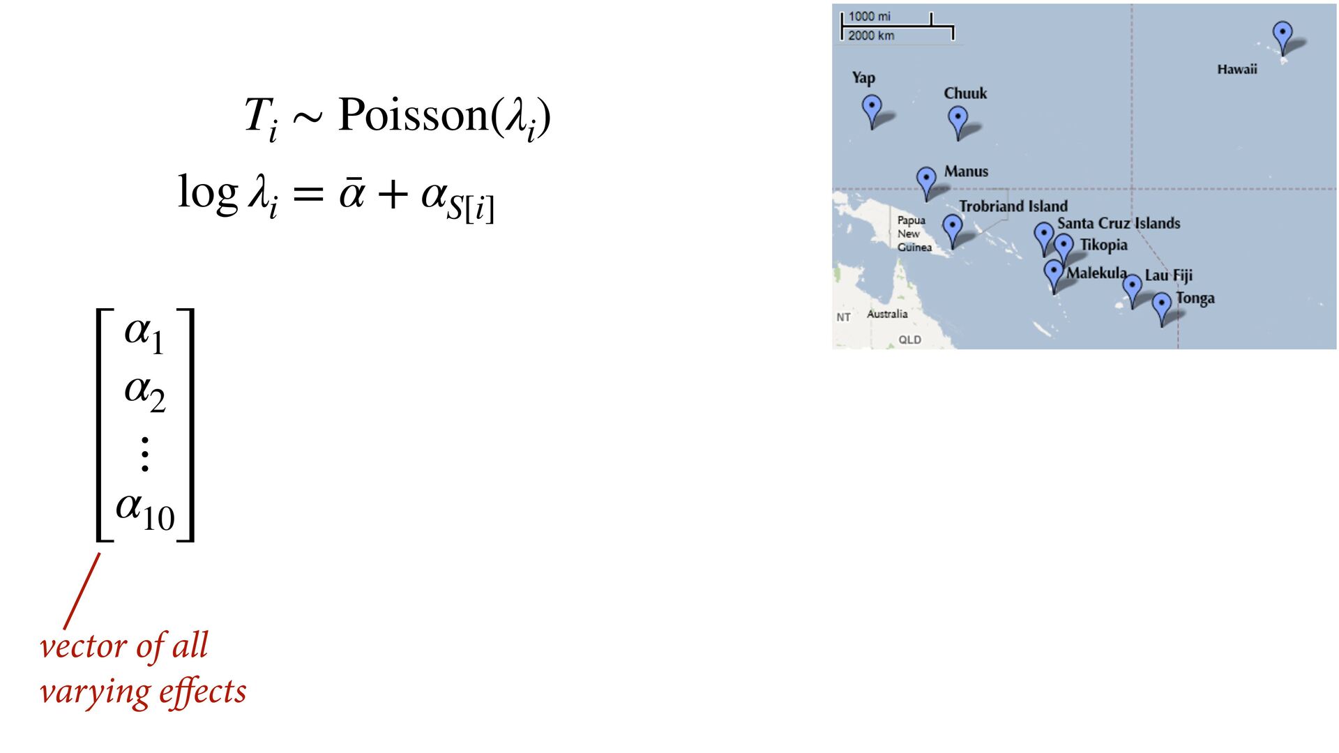
![log λ i = ¯ α + α S[i] T](https://files.speakerdeck.com/presentations/ac82407e9778495caf907541e0c9c5cf/slide_11.jpg)
![log λ i = ¯ α + α S[i] T](https://files.speakerdeck.com/presentations/ac82407e9778495caf907541e0c9c5cf/slide_25.jpg)
![log λ i = ¯ α + α S[i] T](https://files.speakerdeck.com/presentations/ac82407e9778495caf907541e0c9c5cf/slide_26.jpg)
![log λ i = ¯ α + α S[i] T](https://files.speakerdeck.com/presentations/ac82407e9778495caf907541e0c9c5cf/slide_28.jpg)