Upgrade to Pro — share decks privately, control downloads, hide ads and more …

Panagiota Filippou

Panagiota Filippou

SAM Conference 2017

July 04, 2017
Tweet

More Decks by SAM Conference 2017

Other Decks in Research

Transcript

  1. Penalized Likelihood Estimation of Trivariate Binary Models Panagiota Filippou 1

    Giampiero Marra 2 Rosalba Radice 3 1,2Department of Statistical Science, University College London 3Department of Economics, Mathematics and Statistics, Birkbeck, University of London July 4, 2017 SAM conference, University of Liverpool
  2. Introduction Aim: estimate a trivariate system of binary regressions which

    accounts for several types of covariate effects (e.g., linear, non-linear and spatial effects) residual dependence between the responses. Example: model jointly multiple births (i.e., twins, triplets, etc.) premature birth (i.e., infant was born before completing the 37 gestational week) low birth weight (i.e., infant’s birth weight is ≤ 2500 grams). Trivariate probit models deal with these problems.
  3. The trivariate probit model y∗ 1i = η1i + ε1i

    = v1i γ1 + ˜ N1 ν1=1 s1ν1 (z1ν1i ) + ε1i y∗ 2i = η2i + ε2i = v2i γ2 + ˜ N2 ν2=1 s2ν2 (z2ν2i ) + ε2i y∗ 3i = η3i + ε3i = v3i γ3 + ˜ N3 ν3=1 s3ν3 (z3ν3i ) + ε3i , i = 1, . . . , n. y∗ mi is a latent continuous variable and ymi = 1(y∗ mi > 0), ∀m = 1, 2, 3. vmi γm and ˜ Nm νm=1 smνm (zmνmi ) refer to parametric and non- parametric components. (ε1i , ε2i , ε3i ) = εi iid ∼ N3(0, Σ), Σ =   1 ϑ12 ϑ13 ϑ21 1 ϑ23 ϑ31 ϑ32 1  .
  4. Estimation Log-likelihood function for the trivariate probit model: (δ) =

    n i=1 {y1i y2i y3i log p111i + y1i y2i ˜ y3i log p110i + y1i ˜ y2i y3i log p101i + ˜ y1i y2i y3i log p011i + ˜ y1i ˜ y2i ˜ y3i log p000i + ˜ y1i y2i ˜ y3i log p010i +˜ y1i ˜ y2i y3i log p001i + y1i ˜ y2i ˜ y3i log p100i } , where ˜ ymi = (1−ymi ), p¯ e1 ¯ e2 ¯ e3 = P(y1i = ¯ e1, y2i = ¯ e2, y3i = ¯ e3), ∀¯ em ∈ {0, 1}, ∀m = 1, 2, 3. Simultaneous estimation of all parameters can be achieved by penalized MLE (PMLE) solving the optimization problem ˆ δ := arg min δ − (δ) − 1 2 δ ˜ Sλδ , where δ ˜ Sλδ is a penalty term that controls for the model’s smoothness and depends on the smoothing parameter λ which controls the trade-off between fit and smoothness.
  5. Simulation results–DGP1 Method Comparison − DGP1 − n = 1000

    −0.9 −0.7 −0.5 mvprobit SemiParTRIV ϑ ^ 12 −0.8−0.6−0.4−0.2 mvprobit SemiParTRIV ϑ ^ 13 0.4 0.6 0.8 1.0 mvprobit SemiParTRIV ϑ ^ 23 −1.8 −1.4 γ ^ 31 1.6 2.0 2.4 γ ^ 32 −2.0 −1.5 −1.0 γ ^ 33 −1.4 −1.0 −0.6 γ ^ 21 −1.8 −1.4 −1.0 γ ^ 22 0.5 1.0 1.5 γ ^ 23 1.41.61.82.0 γ ^ 11 0.6 0.8 1.0 1.2 γ ^ 12 −2.0 −1.5 −1.0 γ ^ 13
  6. Method Comparison − DGP1 − n = 10000 −0.9 −0.7

    −0.5 mvprobit SemiParTRIV ϑ ^ 12 −0.8−0.6−0.4−0.2 mvprobit SemiParTRIV ϑ ^ 13 0.4 0.6 0.8 1.0 mvprobit SemiParTRIV ϑ ^ 23 −1.8 −1.4 γ ^ 31 1.6 2.0 2.4 γ ^ 32 −2.0 −1.5 −1.0 γ ^ 33 −1.4 −1.0 −0.6 γ ^ 21 −1.8 −1.4 −1.0 γ ^ 22 0.5 1.0 1.5 γ ^ 23 1.41.61.82.0 γ ^ 11 0.6 0.8 1.0 1.2 γ ^ 12 −2.0 −1.5 −1.0 γ ^ 13
  7. Simulation results–DGP2 The particular choice of the correlation parameters seemed

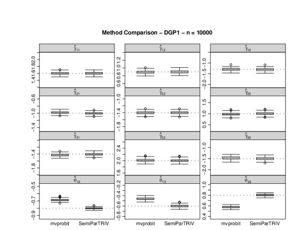
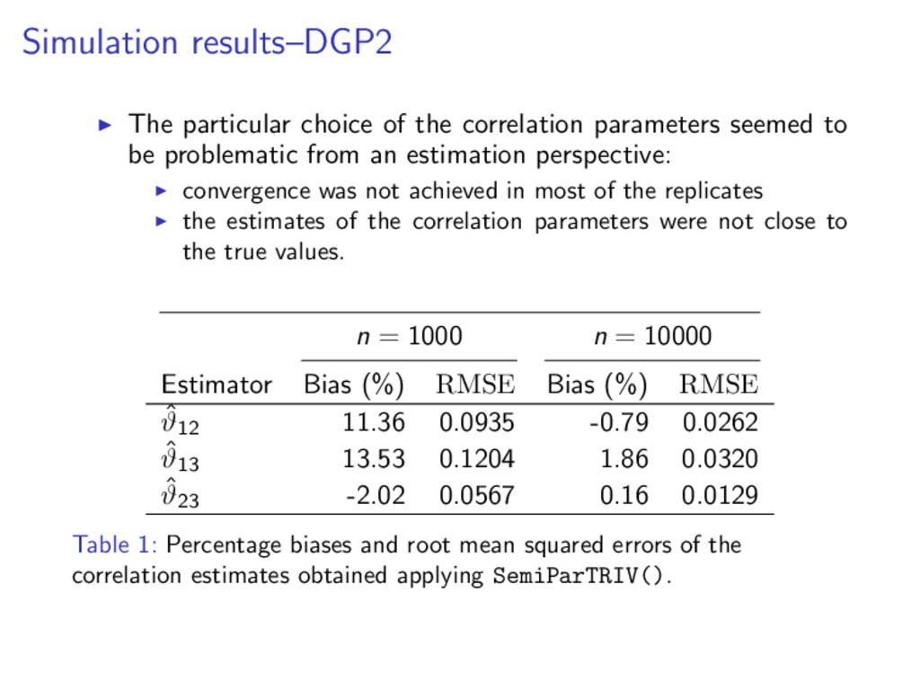
    to be problematic from an estimation perspective: convergence was not achieved in most of the replicates the estimates of the correlation parameters were not close to the true values. n = 1000 n = 10000 Estimator Bias (%) RMSE Bias (%) RMSE ˆ ϑ12 11.36 0.0935 -0.79 0.0262 ˆ ϑ13 13.53 0.1204 1.86 0.0320 ˆ ϑ23 -2.02 0.0567 0.16 0.0129 Table 1: Percentage biases and root mean squared errors of the correlation estimates obtained applying SemiParTRIV().
  8. Correlation-based penalty The issue with estimating the correlation parameters can

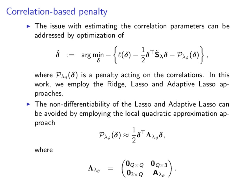
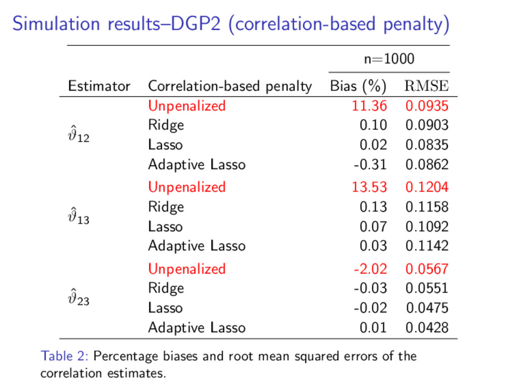
    be addressed by optimization of ˆ δ := arg min δ − (δ) − 1 2 δ ˜ Sλδ − Pλϑ (δ) , where Pλϑ (δ) is a penalty acting on the correlations. In this work, we employ the Ridge, Lasso and Adaptive Lasso ap- proaches. The non-differentiability of the Lasso and Adaptive Lasso can be avoided by employing the local quadratic approximation ap- proach Pλϑ (δ) ≈ 1 2 δ Λλϑ δ, where Λλϑ = 0Q×Q 0Q×3 03×Q Aλϑ .
  9. Simulation results–DGP2 (correlation-based penalty) n=1000 Estimator Correlation-based penalty Bias (%)

    RMSE ˆ ϑ12 Unpenalized 11.36 0.0935 Ridge 0.10 0.0903 Lasso 0.02 0.0835 Adaptive Lasso -0.31 0.0862 ˆ ϑ13 Unpenalized 13.53 0.1204 Ridge 0.13 0.1158 Lasso 0.07 0.1092 Adaptive Lasso 0.03 0.1142 ˆ ϑ23 Unpenalized -2.02 0.0567 Ridge -0.03 0.0551 Lasso -0.02 0.0475 Adaptive Lasso 0.01 0.0428 Table 2: Percentage biases and root mean squared errors of the correlation estimates.
  10. Case study The data set consists of 61,426 female newborns

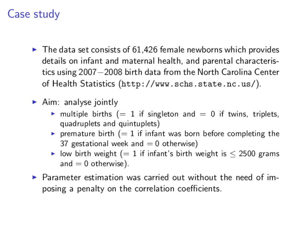
    which provides details on infant and maternal health, and parental characteris- tics using 2007−2008 birth data from the North Carolina Center of Health Statistics (http://www.schs.state.nc.us/). Aim: analyse jointly multiple births (= 1 if singleton and = 0 if twins, triplets, quadruplets and quintuplets) premature birth (= 1 if infant was born before completing the 37 gestational week and = 0 otherwise) low birth weight (= 1 if infant’s birth weight is ≤ 2500 grams and = 0 otherwise). Parameter estimation was carried out without the need of im- posing a penalty on the correlation coefficients.
  11. Case study results SemiParTRIV() mvprobit() ˆ ϑ12 -0.7617 (-0.7612, -0.7622)

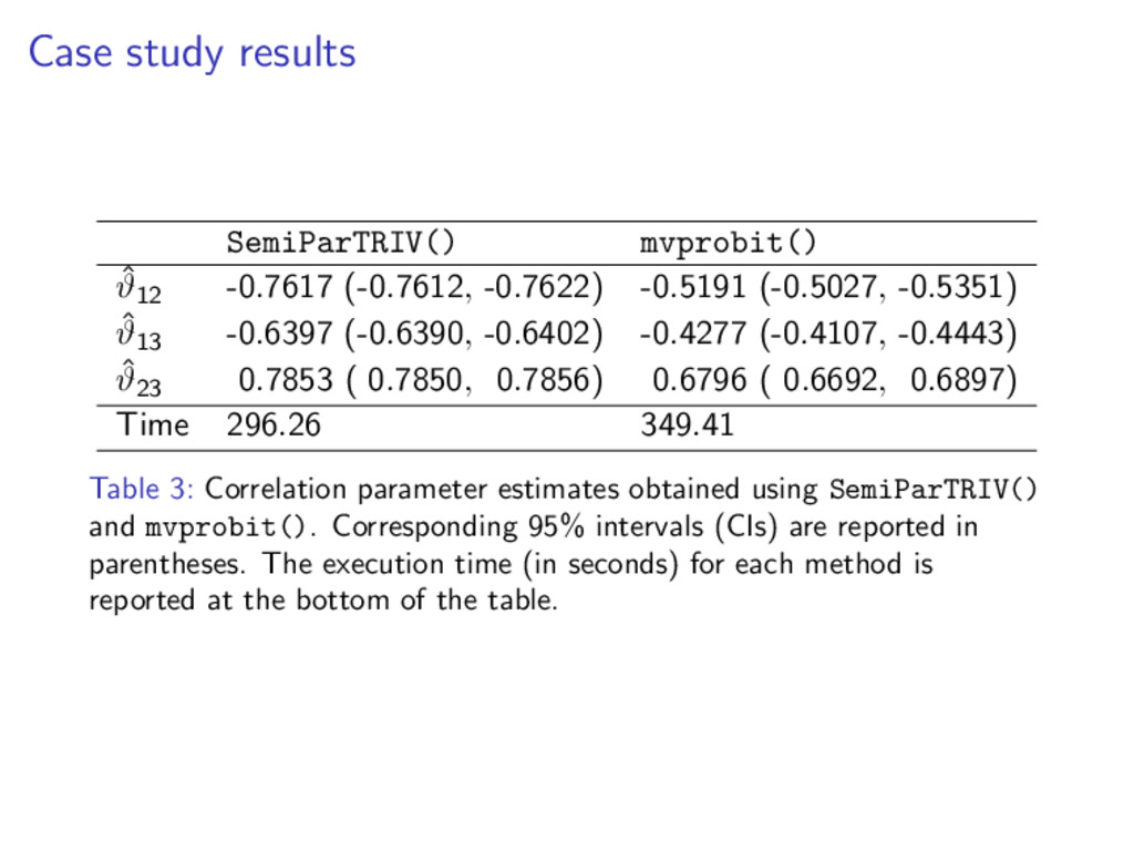
    -0.5191 (-0.5027, -0.5351) ˆ ϑ13 -0.6397 (-0.6390, -0.6402) -0.4277 (-0.4107, -0.4443) ˆ ϑ23 0.7853 ( 0.7850, 0.7856) 0.6796 ( 0.6692, 0.6897) Time 296.26 349.41 Table 3: Correlation parameter estimates obtained using SemiParTRIV() and mvprobit(). Corresponding 95% intervals (CIs) are reported in parentheses. The execution time (in seconds) for each method is reported at the bottom of the table.
  12. Case study results (continued) 0.5 1.0 1.5 SemiParTRIV 0.5 1.0

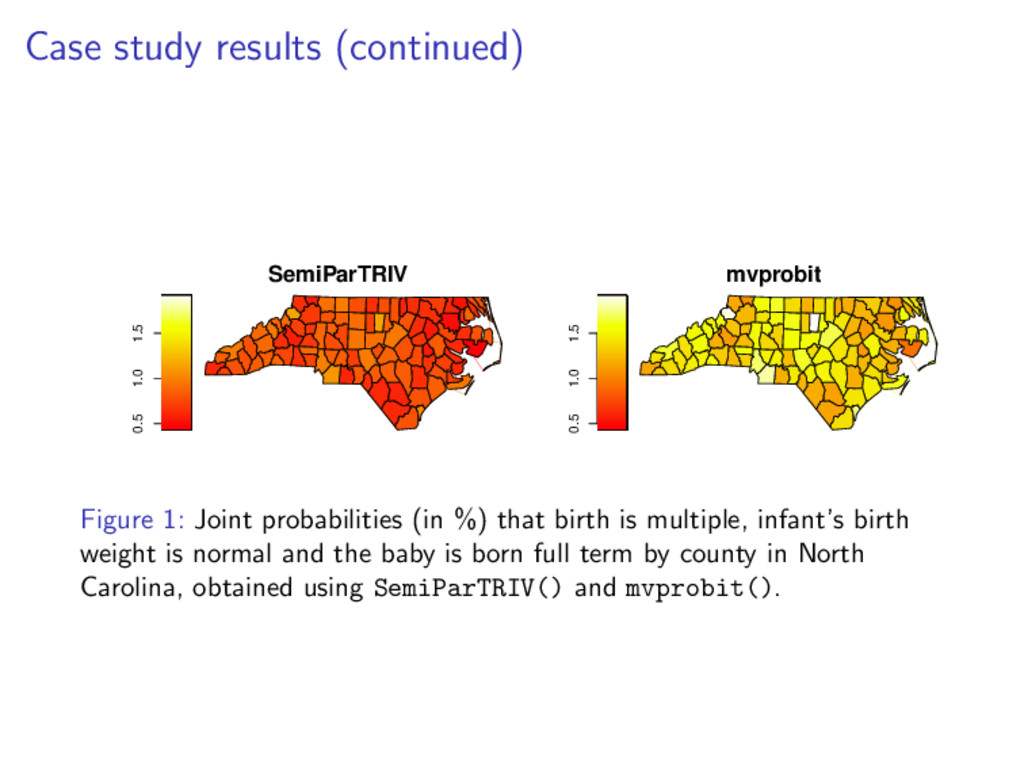
    1.5 mvprobit Figure 1: Joint probabilities (in %) that birth is multiple, infant’s birth weight is normal and the baby is born full term by county in North Carolina, obtained using SemiParTRIV() and mvprobit().
  13. Extending the trivariate probit model Extension I: Modelling unobserved confounders:

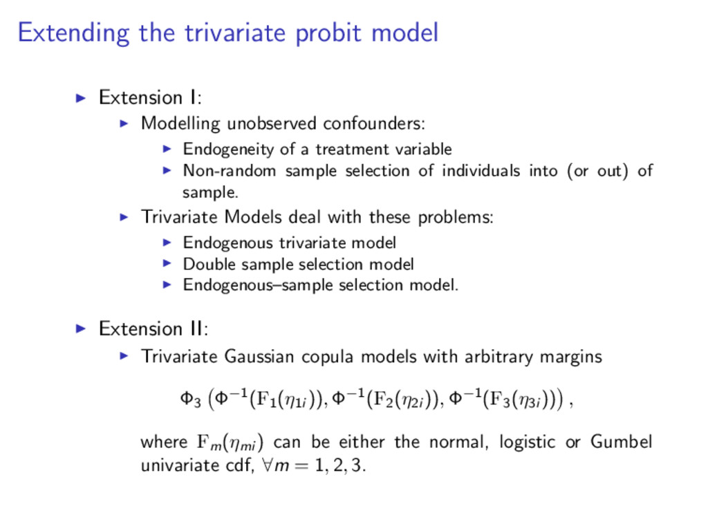
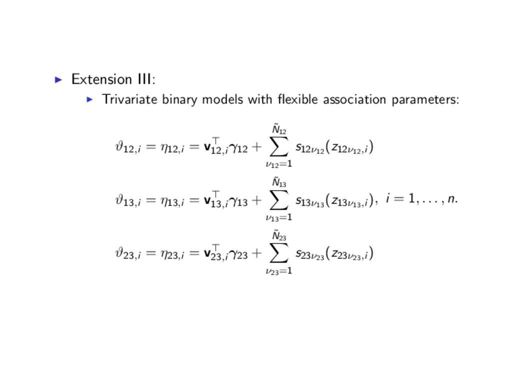
    Endogeneity of a treatment variable Non-random sample selection of individuals into (or out) of sample. Trivariate Models deal with these problems: Endogenous trivariate model Double sample selection model Endogenous–sample selection model. Extension II: Trivariate Gaussian copula models with arbitrary margins Φ3 Φ−1(F1 (η1i )), Φ−1(F2 (η2i )), Φ−1(F3 (η3i )) , where Fm (ηmi ) can be either the normal, logistic or Gumbel univariate cdf, ∀m = 1, 2, 3.
  14. Extension III: Trivariate binary models with flexible association parameters: ϑ12,i

    = η12,i = v12,i γ12 + ˜ N12 ν12=1 s12ν12 (z12ν12,i ) ϑ13,i = η13,i = v13,i γ13 + ˜ N13 ν13=1 s13ν13 (z13ν13,i ) ϑ23,i = η23,i = v23,i γ23 + ˜ N23 ν23=1 s23ν23 (z23ν23,i ) , i = 1, . . . , n.
  15. The SemiParTRIV() routine The models can be easily estimated using

    the SemiParTRIV() rou- tine in the R package SemiParBIVProbit: out <- SemiParTRIV(formula = f.l, data = dat, margins = marg, Model = mod, penCor = PenFun) where f.l <- list(eqn1, eqn2, eqn3, eqn4, eqn5, eqn6) eqn1 <- y1 ~ v1 + z1; eqn2 <- y2 ~ v2 + z2; eqn3 <- y3 ~ v3 + z3; eqn4 <- ~ v1 + z1; eqn5 <- ~ v2 + z2; eqn6 <- ~ v3 + z3 marg <- c("probit", "logit", "cloglog") mod <- "T"; mod <- "TSS"; mod <- "ESS" PenFun <- "ridge"; PenFun <- "lasso"; PenFun <- "alasso"