Structures de Données Exotiques

Devoxx France 2013 Conference, on advanced data structures.
SkipLists
Hash Array Mapped Tries
Bloom Filters
Count min sketch

Transcript

1. 17h - 17h50 - Salle Seine A
   STRUCTURES DE DONNEES
   EXOTIQUES
   

   View Slide

2. • Sam BESSALAH
   
   
   
   • Independent Software Developer,
   
   
   
   • Works for startups, finance shops, mostly in Big
   Data, Machine Learning related projects.
   
   
   
   • Rambling on twitter as @samklr
   
   

   View Slide

3. Why care about data structures?
   
   
   

   View Slide

4. Powerful librairies, powerful frameworks.
   
   
   But ..
   
   
   
   
   
   
   « If all you have is a hammer, everything looks
   
   like a nail ».
   
   
   Abraham H. Maslow
   
   
   
   
   

   View Slide

5. SKIPLISTS
   
   
   

   View Slide

6. Efficient structure for sorted data sets
   
   
   
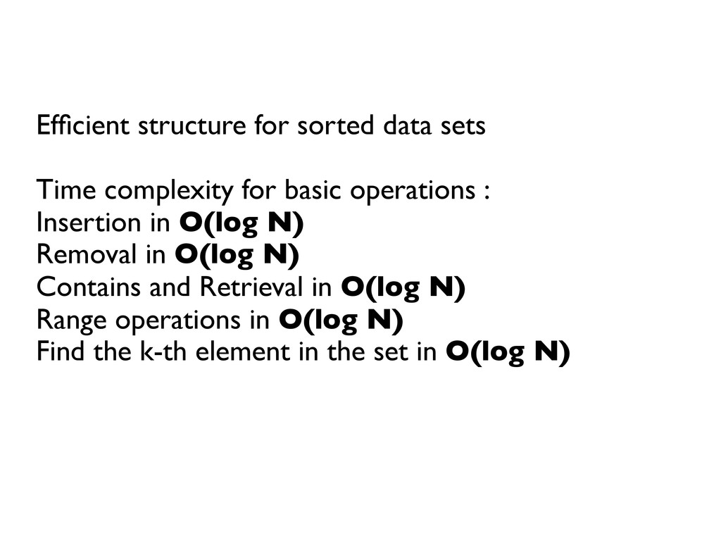
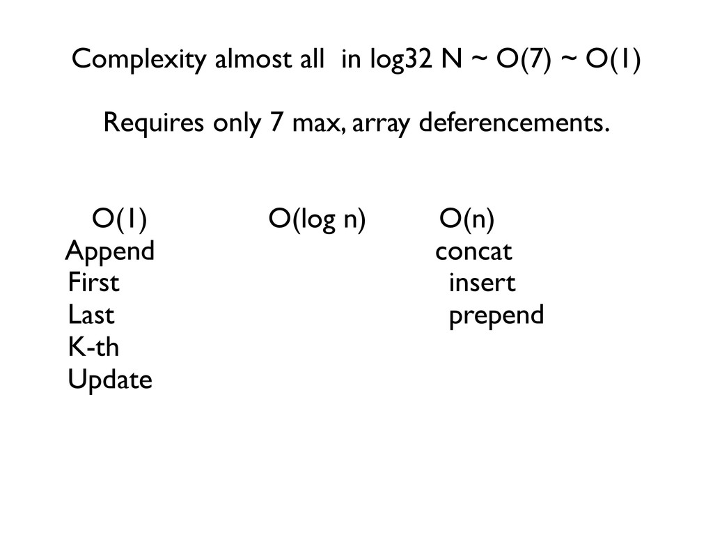
   Time complexity for basic operations :
   
   Insertion in O(log N)
   
   Removal in O(log N)
   
   Contains and Retrieval in O(log N)
   
   Range operations in O(log N)
   
   Find the k-th element in the set in O(log N)
   
   
   
   

   View Slide

7. Start with a simple linked list
   

   View Slide

8. Add extra levels for express lines
   

   View Slide

9. Search for a value looks like this
   

   View Slide

10. 
    
    Insert (X)
    
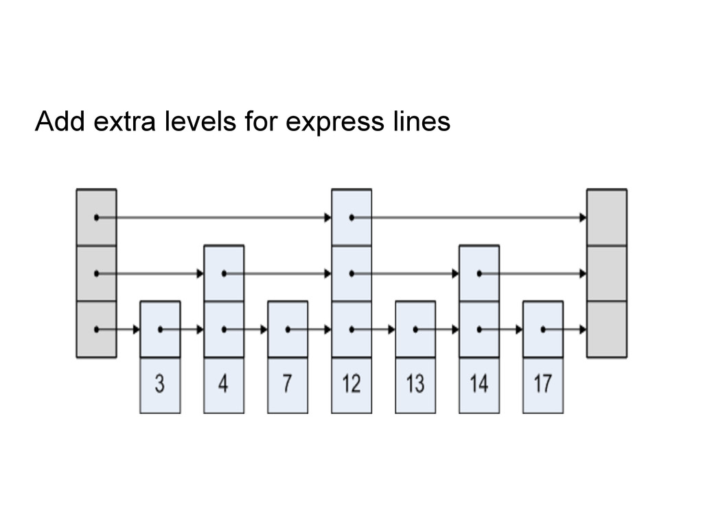
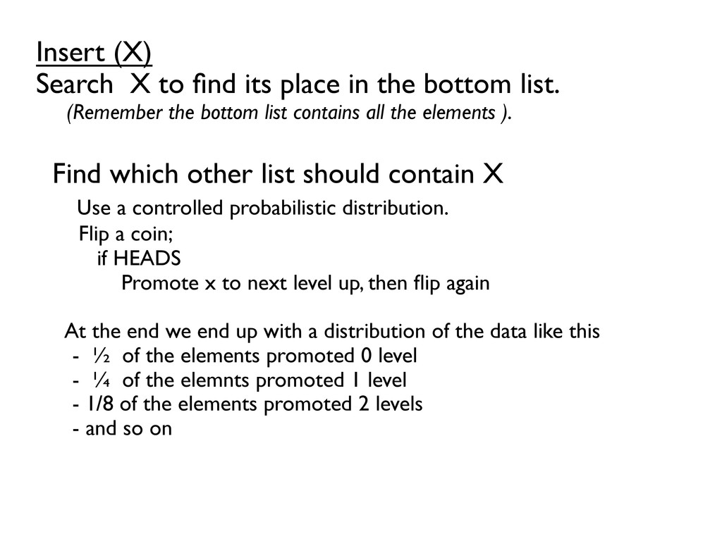
    Search X to find its place in the bottom list.
    
    (Remember the bottom list contains all the elements ).
    
    
    
    Find which other list should contain X
    
    Use a controlled probabilistic distribution.
    
    Flip a coin;
    
    if HEADS
    
    Promote x to next level up, then flip again
    
    
    
    At the end we end up with a distribution of the data like this
    
    - ½ of the elements promoted 0 level
    
    - ¼ of the elemnts promoted 1 level
    
    - 1/8 of the elements promoted 2 levels
    
    - and so on
    
    

    View Slide

11. Remove (X)
    
    Find X in all the levels it participates and delete
    
    If One or more of the upper levels are empty,
    remove them.
    

    View Slide

12. Insert
    
    void insert(E value) {
    SkipNode x = header;
    SkipNode[] update = new SkipNode[MAX_LEVEL + 1];
    for (int i = level; i >= 0; i--) {
    while (x.forward[i] != null && x.forward[i].value.compareTo(value) < 0) {
    x = x.forward[i];
    }
    update[i] = x;
    }
    x = x.forward[0];
    if (x == null || !x.value.equals(value)) {
    int lvl = randomLevel();
    if (lvl > level) {
    for (int i = level + 1; i <= lvl; i++) {
    update[i] = header;
    }
    level = lvl;
    }
    

    View Slide

13. …
    
    x = new SkipNode(lvl, value);
    for (int i = 0; i <= lvl; i++) {
    x.forward[i] = update[i].forward[i];
    update[i].forward[i] = x; }
    }
    }
    private int getLevel(){ // Coin Flipping
    int lvl = (int)(Math.log(1.-Math.random())/Math.log(1.-P));
    return Math.min(lvl, MAX_LEVEL);
    }
    

    View Slide

14. Fast structure on average, very fast in practice
    
    
    
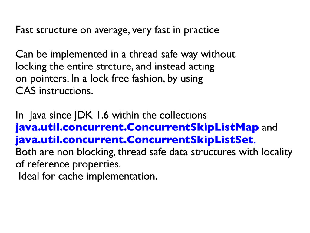
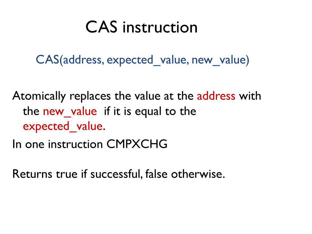
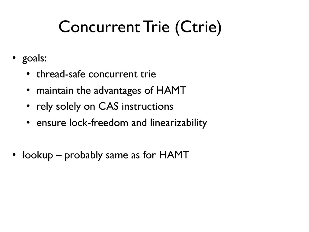
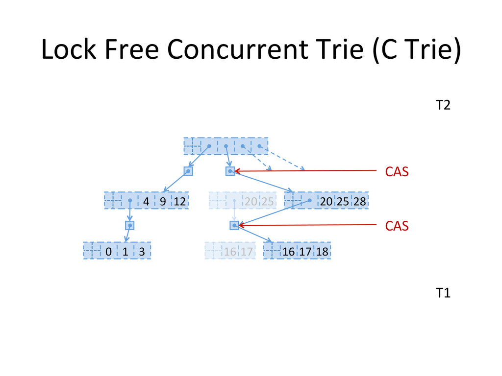
    Can be implemented in a thread safe way without
    
    locking the entire strcture, and instead acting
    
    on pointers. In a lock free fashion, by using
    
    CAS instructions.
    
    
    
    In Java since JDK 1.6 within the collections
    java.util.concurrent.ConcurrentSkipListMap and
    
    java.util.concurrent.ConcurrentSkipListSet.
    
    Both are non blocking, thread safe data structures with locality
    of reference properties.
    
    Ideal for cache implementation.
    
    

    View Slide

15. CAS instruction
    
    CAS(address, expected_value, new_value)
    
    
    
    Atomically replaces the value at the address with
    the new_value if it is equal to the
    expected_value.
    
    In one instruction CMPXCHG
    
    
    
    Returns true if successful, false otherwise.
    
    
    
    
    
    

    View Slide

16. Drawbacks
    They can be memory hungry, by being space
    inefficient.
    

    View Slide

17. TRIES
    
    
    

    View Slide

18. 
    
    - Ordered Tree data structure, used to store associative
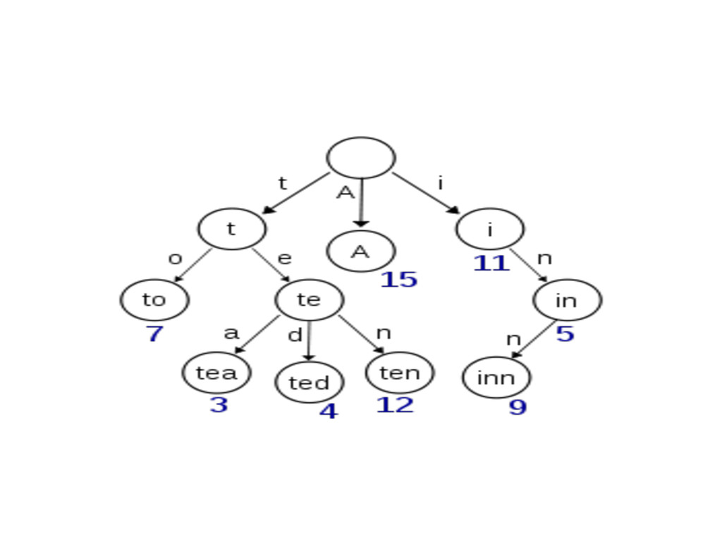
    arrays. Usually, encoded keys through traversal, in the nodes of
    the tree with value in the leaves.
    
    
    
    -Used for dictionnary (Map), word completion,
    
    web requests parsing., etc.
    
    
    
    -Time complexity in O(k) where k is the length of
    
    searched string. Where it usually is O(length of the tree)
    
    
    
    
    
    

    View Slide

19. View Slide

20. HASH ARRAY MAPPED TRIE

    View Slide

21. View Slide

22. How does it work?
    
    
    
    
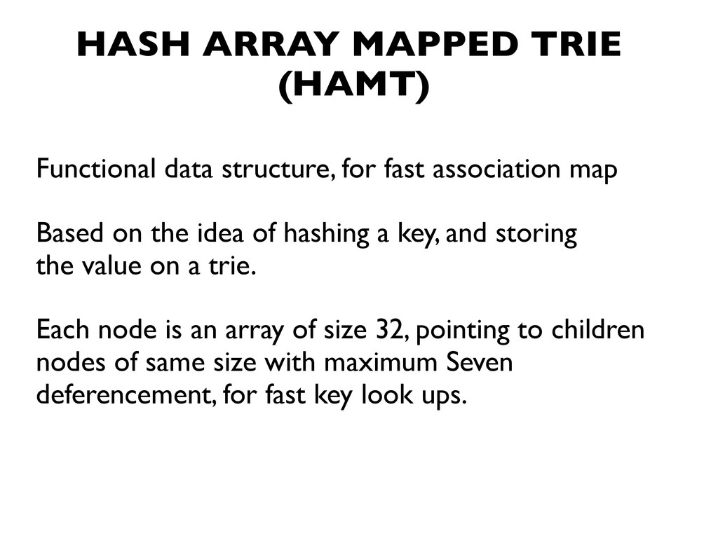
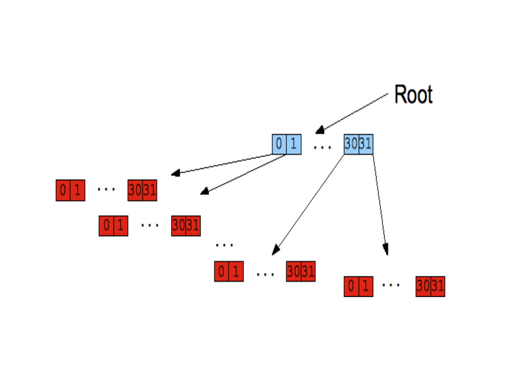
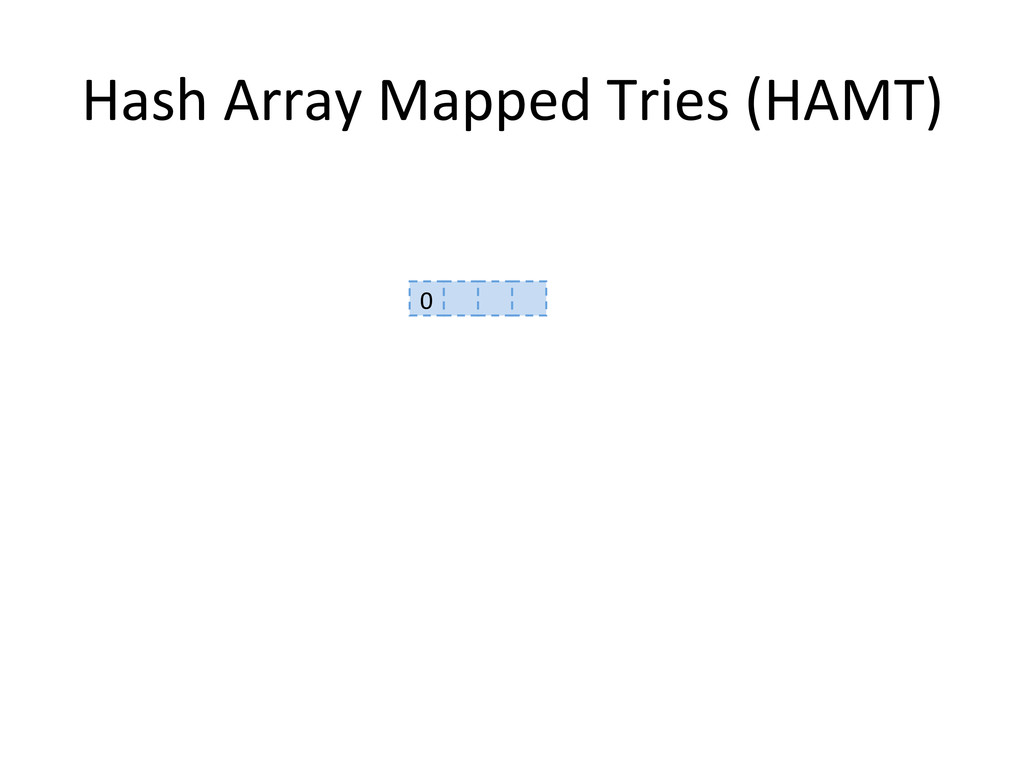
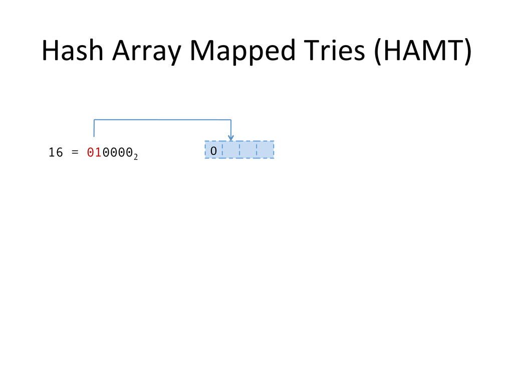
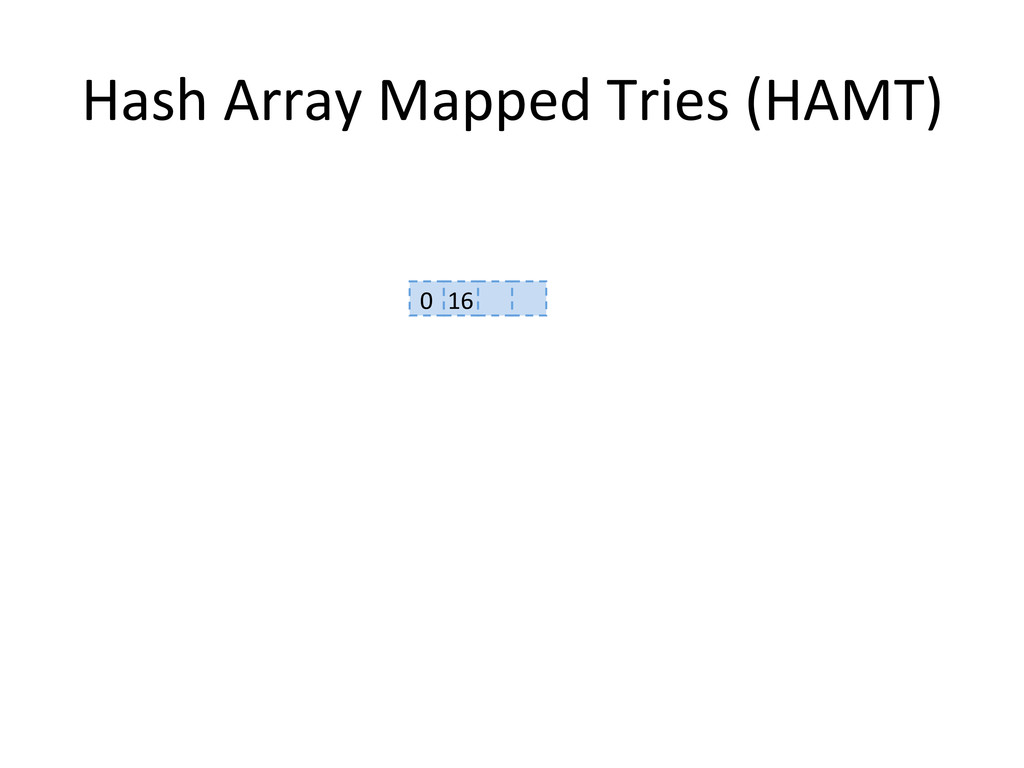
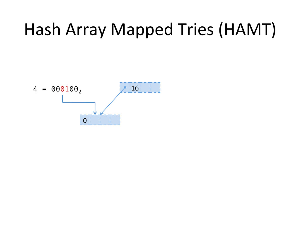
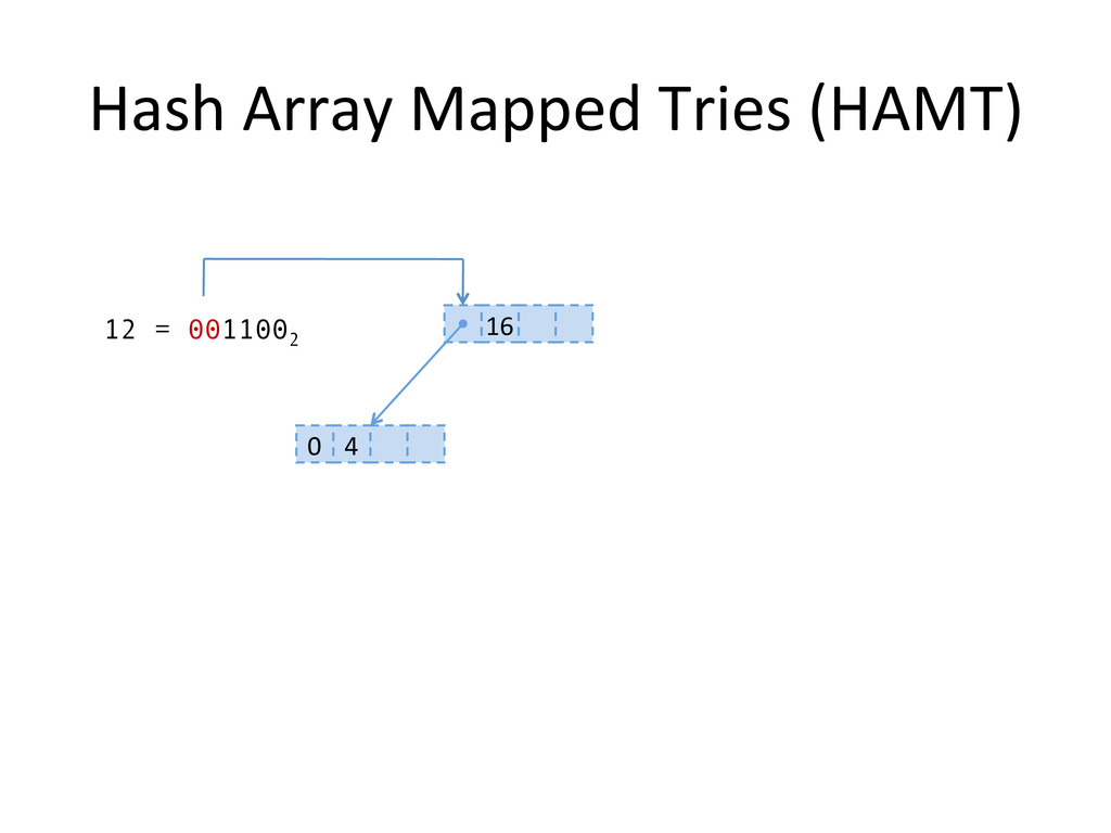
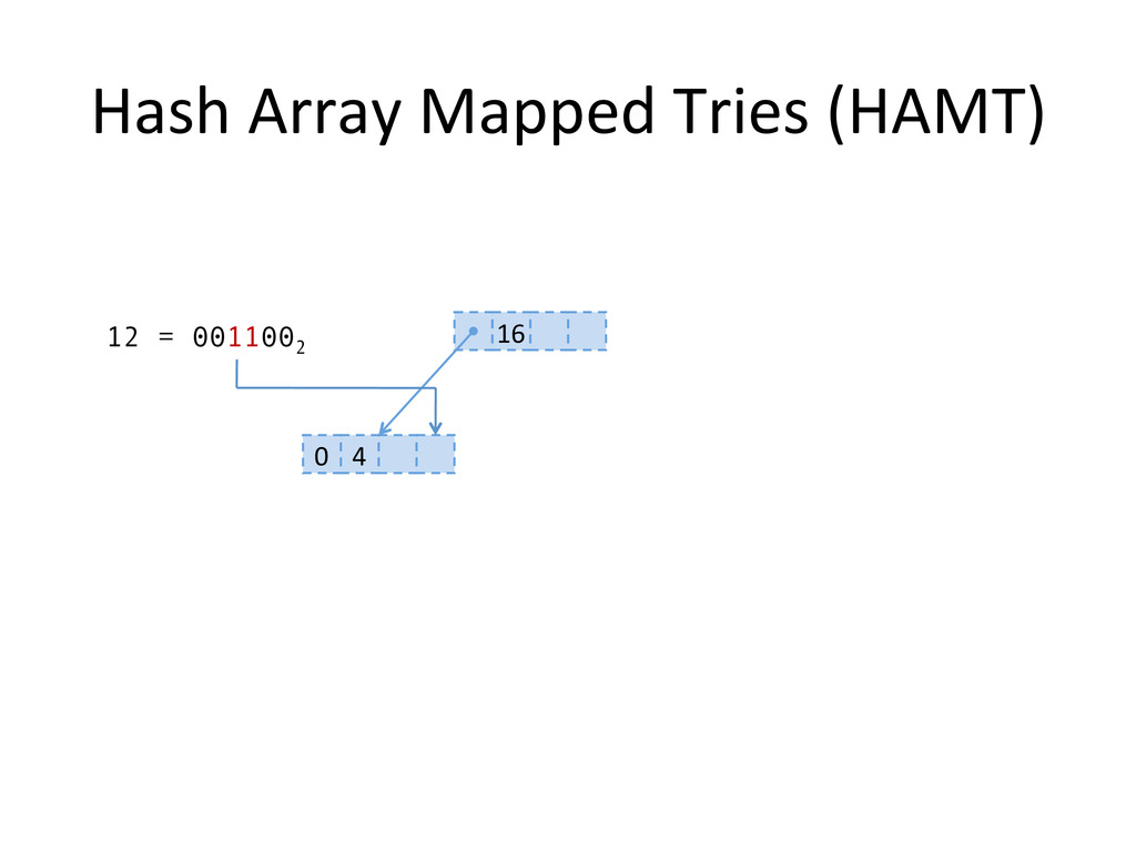
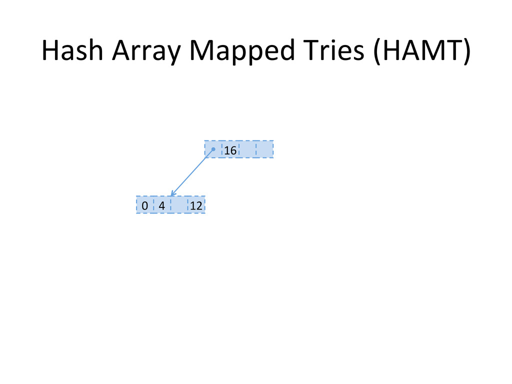
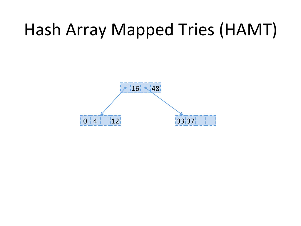
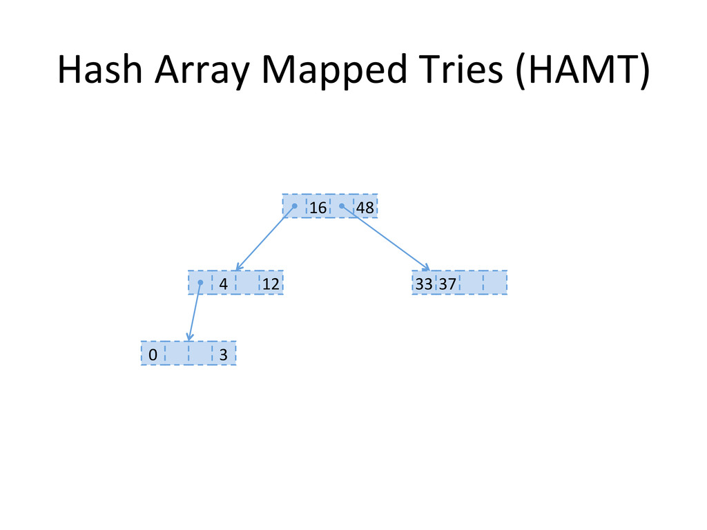
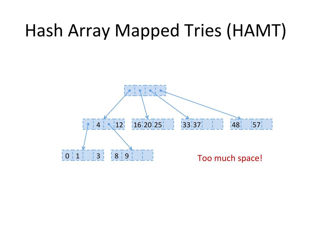
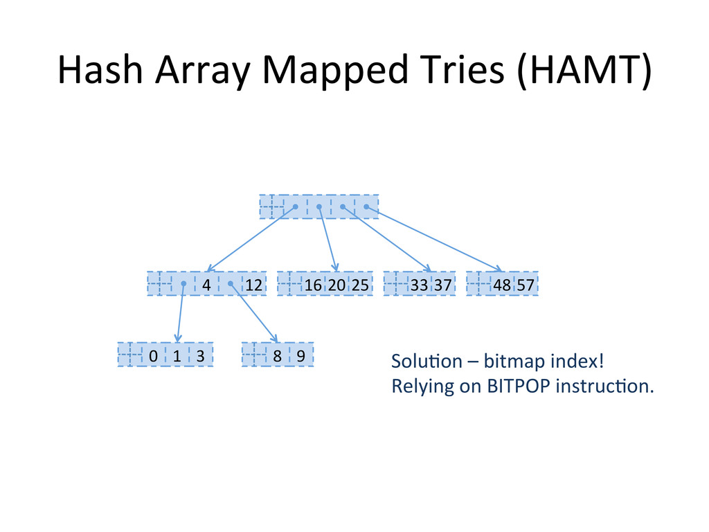
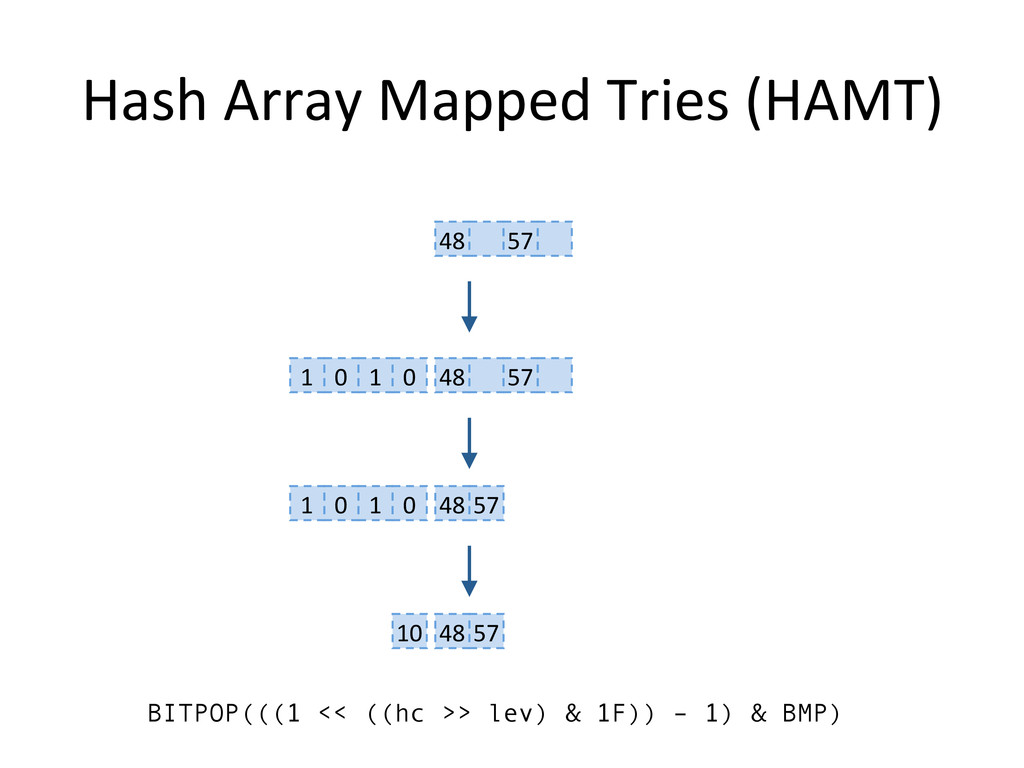
    During association of K → V , compute hashes yielding an Integer
    or a long, coded on the JVM in 32 bits
    
    
    
    Partition those bits to blocks of 5 bits, representing
    
    a level in the tree structure, from the right most (root)
    
    to the left most (leaves)
    
    
    
    The colored nodes have between 2 and 31 children
    
    
    
    Each colored node maintain a bitmap, encoding
    
    how many children the nodes contains, and their indexes
    
    in the array.
    
    

    View Slide

23. Trie Structure (from Rich Hikey)
    

    View Slide

24. Hash  Array  Mapped  Tries  (HAMT)  
    

    View Slide

25. Hash  Array  Mapped  Tries  (HAMT)  
    0 = 0000002
    

    View Slide

26. Hash  Array  Mapped  Tries  (HAMT)  
    0  
    

    View Slide

27. Hash  Array  Mapped  Tries  (HAMT)  
    0  
    16 = 0100002
    

    View Slide

28. Hash  Array  Mapped  Tries  (HAMT)  
    0   16  
    

    View Slide

29. Hash  Array  Mapped  Tries  (HAMT)  
    0   16  
    4 = 0001002
    

    View Slide

30. Hash  Array  Mapped  Tries  (HAMT)  
    16  
    0  
    4 = 0001002
    

    View Slide

31. Hash  Array  Mapped  Tries  (HAMT)  
    16  
    0   4  
    

    View Slide

32. Hash  Array  Mapped  Tries  (HAMT)  
    16  
    0   4  
    12 = 0011002
    

    View Slide

33. Hash  Array  Mapped  Tries  (HAMT)  
    16  
    0   4  
    12 = 0011002
    

    View Slide

34. Hash  Array  Mapped  Tries  (HAMT)  
    16  
    0   4   12  
    

    View Slide

35. Hash  Array  Mapped  Tries  (HAMT)  
    16  33  
    0   4   12  
    

    View Slide

36. Hash  Array  Mapped  Tries  (HAMT)  
    16  33  
    0   4   12  
    48  
    

    View Slide

37. Hash  Array  Mapped  Tries  (HAMT)  
    16  
    0   4   12  
    48  
    33  37  
    

    View Slide

38. Hash  Array  Mapped  Tries  (HAMT)  
    16  
    4   12  
    48  
    33  37  
    0   3  
    

    View Slide

39. Hash  Array  Mapped  Tries  (HAMT)  
    4   12   16  20  25   33  37  
    0   1   8   9  
    3  
    48   57  
    

    View Slide

40. Hash  Array  Mapped  Tries  (HAMT)  
    4   12   16  20  25   33  37  
    0   1   8   9  
    3  
    48   57  
    Too  much  space!  
    

    View Slide

41. Hash  Array  Mapped  Tries  (HAMT)  
    4   12   16  20  25   33  37  
    0   1   8   9  
    3  
    48  57  
    

    View Slide

42. Hash  Array  Mapped  Tries  (HAMT)  
    4   12   16  20  25   33  37  
    0   1   8   9  
    3  
    48  57  
    Linear  search  at  every  level  -­‐  slow!  
    

    View Slide

43. Hash  Array  Mapped  Tries  (HAMT)  
    4   12   16  20  25   33  37  
    0   1   8   9  
    3  
    48  57  
    SoluHon  –  bitmap  index!  
    Relying  on  BITPOP  instrucHon.  
    

    View Slide

44. Hash  Array  Mapped  Tries  (HAMT)  
    48   57  
    48   57  
    1   0   1   0  
    48  57  
    1   0   1   0  
    48  57  
    10  
    BITPOP(((1 << ((hc >> lev) & 1F)) – 1) & BMP)
    

    View Slide

45. Complexity almost all in log32 N ~ O(7) ~ O(1)
    
    
    
    
    Requires only 7 max, array deferencements.
    
    
    
    
    
    
    O(1) O(log n) O(n)
    
    Append concat
    
    First
    
    
    
    
    
    
    
    
    
    
    insert
    
    Last
    
    
    
    
    
    
    
    
    
    
    prepend
    
    K-th
    
    Update
    
    

    View Slide

46. Hash Array Mapped Tries
    (HAMT)
    •  advantages:
    
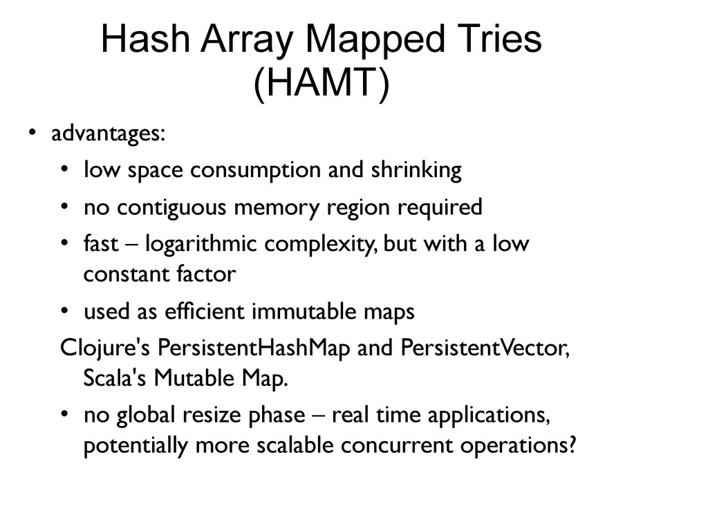
    •  low space consumption and shrinking
    
    •  no contiguous memory region required
    
    •  fast – logarithmic complexity, but with a low
    constant factor
    
    •  used as efficient immutable maps
    
    Clojure's PersistentHashMap and PersistentVector,
    Scala's Mutable Map.
    
    •  no global resize phase – real time applications,
    potentially more scalable concurrent operations?
    
    

    View Slide

47. Concurrent Trie (Ctrie)
    
    •  goals:
    
    •  thread-safe concurrent trie
    
    •  maintain the advantages of HAMT
    
    •  rely solely on CAS instructions
    
    •  ensure lock-freedom and linearizability
    
    
    
    •  lookup – probably same as for HAMT
    
    

    View Slide

48. Lock  Free  Concurrent  Trie  (C  Trie)  
    4   9   12  
    0   1   3   16  17  
    T1  
    T2  
    20  25  
    16  17  18  
    20  25  28  
     CAS  
     CAS  
    

    View Slide

49. SKETCHES
    
    
    (Or how to remove the fat in your datasets)
    
    
    

    View Slide

50. BLOOM FILTERS
    
    
    

    View Slide

51. Probabilistic data structures, designed to tell rapidly in a
    
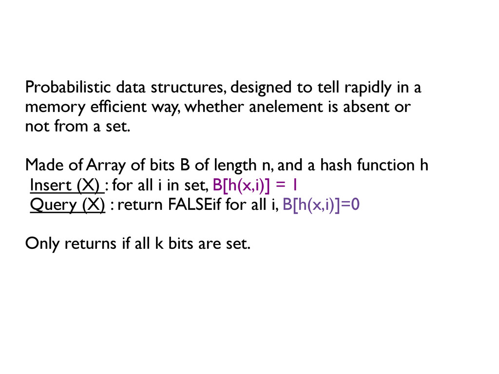
    memory efficient way, whether anelement is absent or
    
    not from a set.
    
    
    
    Made of Array of bits B of length n, and a hash function h
    
    Insert (X) : for all i in set, B[h(x,i)] = 1
    
    Query (X) : return FALSEif for all i, B[h(x,i)]=0
    
    
    
    Only returns if all k bits are set.
    
    
    
    

    View Slide

52. We can pick the error rate and optimize the size of the filter to match requirements.
    
    

    View Slide

53. TRADE OFFS
    
    
    
    More hashes enduce more accurate results, but render the
    sketch less space efficient.
    
    
    
    Choice of the hash function is important.
    
    
    
    Cryptographic hashes are great; because evenly distributed,
    with less collisions.
    
    
    
    Watch out to time spent computing your hashes.
    
    
    
    
    
    
    
    

    View Slide

54. Cool properties
    
    
    
    Intersection and Union through AND and OR bitwise
    operations
    
    
    
    No False negatives
    
    
    
    For union, helps with parallel construction of BF
    
    
    
    Fast approximation of set union, by using bit map instead of
    set manipulation
    
    
    
    
    
    

    View Slide

55. Handling Deletion
    
    
    Bloom filters can handle insertions, but not
    deletions.
    
    
    
    
    
    
    
    If deleting xi
    means resetting 1s to 0s, then
    deleting xi
    will “delete” xj
    .
    
    Solution : Counting Bloom Filter
    
    
    
    0 1 0 0 1 0 1 0 0 1 1 1 0 1 1 0
    B
    xi
    xj
    

    View Slide

56. COUNTING BLOOM FILTERS
    
    
    Keeps track of inserts
    
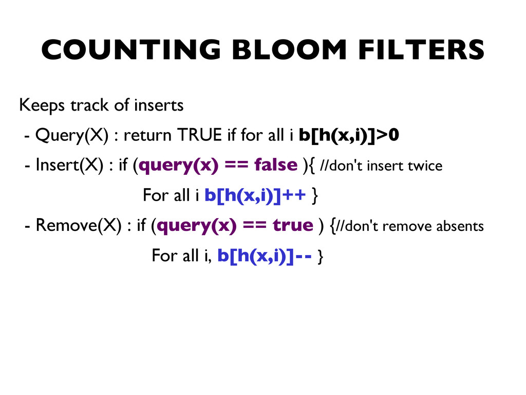
    - Query(X) : return TRUE if for all i b[h(x,i)]>0
    
    - Insert(X) : if (query(x) == false ){ //don't insert twice
    
    For all i b[h(x,i)]++ }
    
    - Remove(X) : if (query(x) == true ) {//don't remove absents
    
    For all i, b[h(x,i)]-- }
    
    

    View Slide

57. Usages
    
    
    - Fast web events tracking
    
    - IO optimisations in databases like Cassandra
    
    Hadoop, Hbases ..
    
    - Network IP filtering ...
    

    View Slide

58. 
    
    Guava Bloom Filters
    
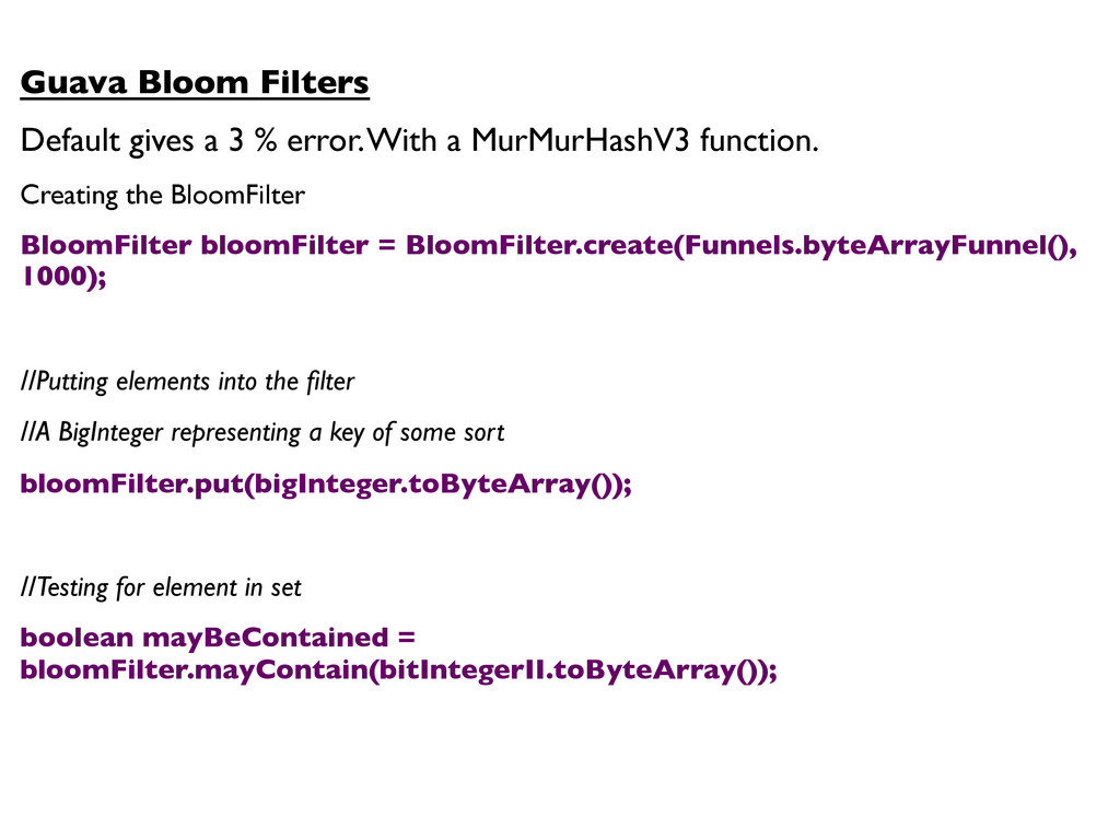
    Default gives a 3 % error. With a MurMurHashV3 function.
    
    Creating the BloomFilter
    
    BloomFilter bloomFilter = BloomFilter.create(Funnels.byteArrayFunnel(),
    1000);
    
    
    
    //Putting elements into the filter
    
    //A BigInteger representing a key of some sort
    
    bloomFilter.put(bigInteger.toByteArray());
    
    
    
    //Testing for element in set
    
    boolean mayBeContained =
    bloomFilter.mayContain(bitIntegerII.toByteArray());
    
    
    
    

    View Slide

59. //With a custom filter
    
    class BigIntegerFunnel implements Funnel {
    
    @Override
    
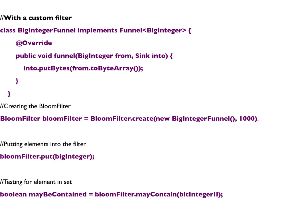
    public void funnel(BigInteger from, Sink into) {
    
    into.putBytes(from.toByteArray());
    
    }
    
    }
    
    //Creating the BloomFilter
    
    BloomFilter bloomFilter = BloomFilter.create(new BigIntegerFunnel(), 1000);
    
    
    
    //Putting elements into the filter
    
    bloomFilter.put(bigInteger);
    
    
    
    //Testing for element in set
    
    boolean mayBeContained = bloomFilter.mayContain(bitIntegerII);
    
    

    View Slide

60. COUNT MIN SKETCHES
    
    
    

    View Slide

61. Family of memory efficient data structures, that can
    
    estimate frequency-related properties of the data set.
    
    
    
    Used to find occurrences of an element in a set, in
    
    time / space efficient way, with a tunable accuracy.
    
    
    
    E.g Find heavy hitters elements; perform range queries
    
    (where the goal is to find the sum of frequencies of
    
    Elements in a certain range ), estimate quantiles.
    
    

    View Slide

62. How does it work?

    View Slide

63. Algorithm :
    
    insert(x):
    
    for i =1 to d
    
    M[i,h(x,i)) ++ //Like counting bloom filters
    
    query(x):
    
    return min {h(x,i) for all 1 ≤ i ≤ d}
    
    
    
    

    View Slide

64. Accuracy depends on the ratio between sketch size
    
    and number of expected data. Works better with
    
    Highly uncorrelated, unstructured data.
    
    
    
    For higly skewed data, use noise estimation,
    
    and compute the median estimation
    
    Error Estimation
    
    
    

    View Slide

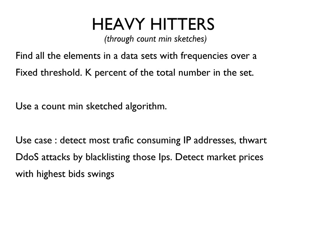
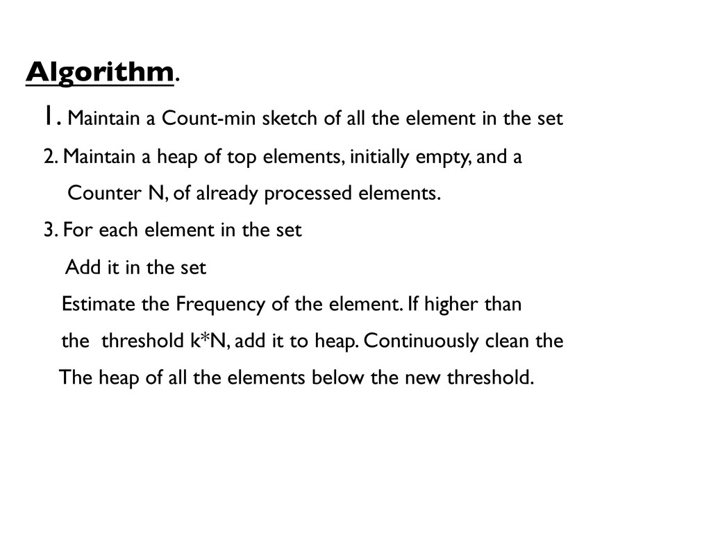
65. Find all the elements in a data sets with frequencies over a
    
    Fixed threshold. K percent of the total number in the set.
    
    
    
    Use a count min sketched algorithm.
    
    
    
    Use case : detect most trafic consuming IP addresses, thwart
    
    DdoS attacks by blacklisting those Ips. Detect market prices
    
    with highest bids swings
    
    HEAVY HITTERS

    View Slide

66. Algorithm.
    
    1. Maintain a Count-min sketch of all the element in the set
    
    2. Maintain a heap of top elements, initially empty, and a
    
    Counter N, of already processed elements.
    
    3. For each element in the set
    
    Add it in the set
    
    Estimate the Frequency of the element. If higher than
    
    the threshold k*N, add it to heap. Continuously clean the
    
    The heap of all the elements below the new threshold.
    
    
    
    

    View Slide

67. OTHER INTERESTING SKETCHES
    
    
    

    View Slide

68. http://highlyscalable.wordpress.com/2012/05/01/probabilistic-
    structures-web-analytics-data-mining/
    

    View Slide

69. Bibliographies & Blogs.
    http://highscalability.com/blog/2012/4/5/big-data-counting-how-to-
    count-a-billion-distinct-objects-us.html
    Librairies. http://github.com/slearspring/stream-lib
    org.apache.cassandra.utils.{MurmurHashV3, BloomFilter}
    Google Guava.
    Ideal Hash Trees by Phil BagWell
    http://infoscience.epfl.ch/record/64398/files/idealhashtrees.pdf
    Concurrent Tries in the Scala Parallel Collections
    SkipLists By William Pugh.
    

    View Slide