Cédric Marchand - Non-Binary LDPC codes

Transcript

1. Non-Binary LDPC codes Cédric Marchand Emmanuel Boutillon name.surname@unv-ubs.fr CNRS, UMR 6285, Lab-STICC Centre de Recherche - BP 92116 F-56321 Lorient Cedex - FRANCE Séminaire CentraleSupélec 3 mars 2016
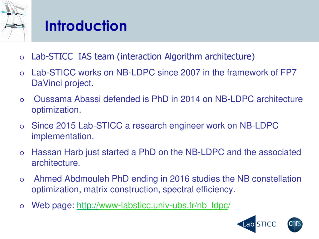
2. Introduction  Lab-STICC IAS team (interaction Algorithm architecture)  Lab-STICC works on NB-LDPC since 2007 in the framework of FP7 DaVinci project.  Oussama Abassi defended is PhD in 2014 on NB-LDPC architecture optimization.  Since 2015 Lab-STICC a research engineer work on NB-LDPC implementation.  Hassan Harb just started a PhD on the NB-LDPC and the associated architecture.  Ahmed Abdmouleh PhD ending in 2016 studies the NB constellation optimization, matrix construction, spectral efficiency.  Web page: http://www-labsticc.univ-ubs.fr/nb_ldpc/
3. OUTLINE 1) Introduction LDPC NB-LDPC Galois Field 2) Decoding NB-LDPC 3) What are the pro and cons of NB-LDPC ?
4. 4 Digital Communication model Source Source Coder Channel Coder Output Source decoder Channel decoder Channel Mapping De-Mapping
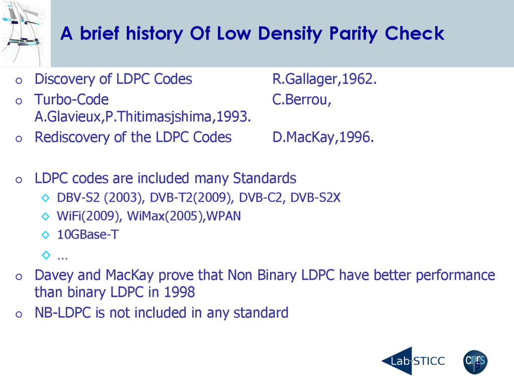
5. 5 A brief history Of Low Density Parity Check  Discovery of LDPC Codes R.Gallager,1962.  Turbo-Code C.Berrou, A.Glavieux,P.Thitimasjshima,1993.  Rediscovery of the LDPC Codes D.MacKay,1996.  LDPC codes are included many Standards ◊ DBV-S2 (2003), DVB-T2(2009), DVB-C2, DVB-S2X ◊ WiFi(2009), WiMax(2005),WPAN ◊ 10GBase-T ◊ …  Davey and MacKay prove that Non Binary LDPC have better performance than binary LDPC in 1998  NB-LDPC is not included in any standard
6. Parity check equation 1 1 1 0 1 0 0 0 1 1 1 0 0 0 1 0 0 0 0 0                 0 4 3 2 1     x x x x          N i i x P 1 2 mod C1 x1 x2 x3 x4 Tanner Graph representation: Variable Node Parity Check Node Examples: Given a word x[x1 x2 x3 x4 ] Edge
7. 7 Parity Check matrix 3 2 1 1 x x x c           1 0 1 0 0 1 1 1 H X1 X2 X3 X4 4 2 2 x x c   The parity check matrix is the set of parity equations: C1 C2 X1 X2 X3 X4 Variable Node Parity Check Node Tanner Graph representation:
8. Decoding  Belief propagation algorithm: ◊ Based on graphical representation of the codes (Tanner graph) ◊ Iterative decoding
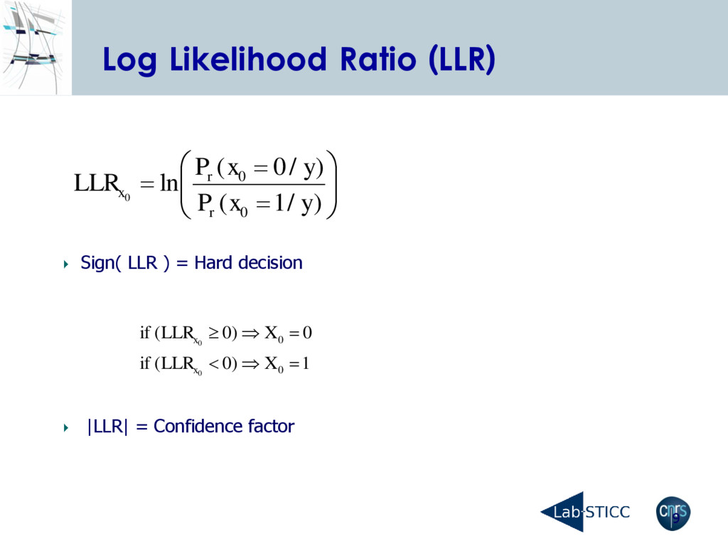
9. 9 Log Likelihood Ratio (LLR)            ) / 1 ( ) / 0 ( ln 0 0 0 y x P y x P LLR r r x 1 ) 0 ( 0 ) 0 ( 0 0 0 0       X LLR if X LLR if x x Sign( LLR ) = Hard decision |LLR| = Confidence factor
10. 10 Belief Propagation algorithm by message passing Channel Input x LLR ( x ) initialization Iterative process – Check Node Update – Variable Node Update Hard Decision making
11. 11 Check node update Mvc Mcv Min-Sum algorithm Normalized Min-Sum algorithm Sub-optimal algorithm +7 +4 + 4 +4 x (0.75)=3
12. 12 Variable node update 1 0    i cv vc M SO M Mcv X0 SO: Soft Output Mvc X0 +2 +1 +3 +7 SO=7+2+1+3 SO=13 Mcv =13-3=10
13. What is a NB-LDPC? It is an LDPC… except that parity check equations are done on a Galois Field GF(q=2m) of cardinality q>2.
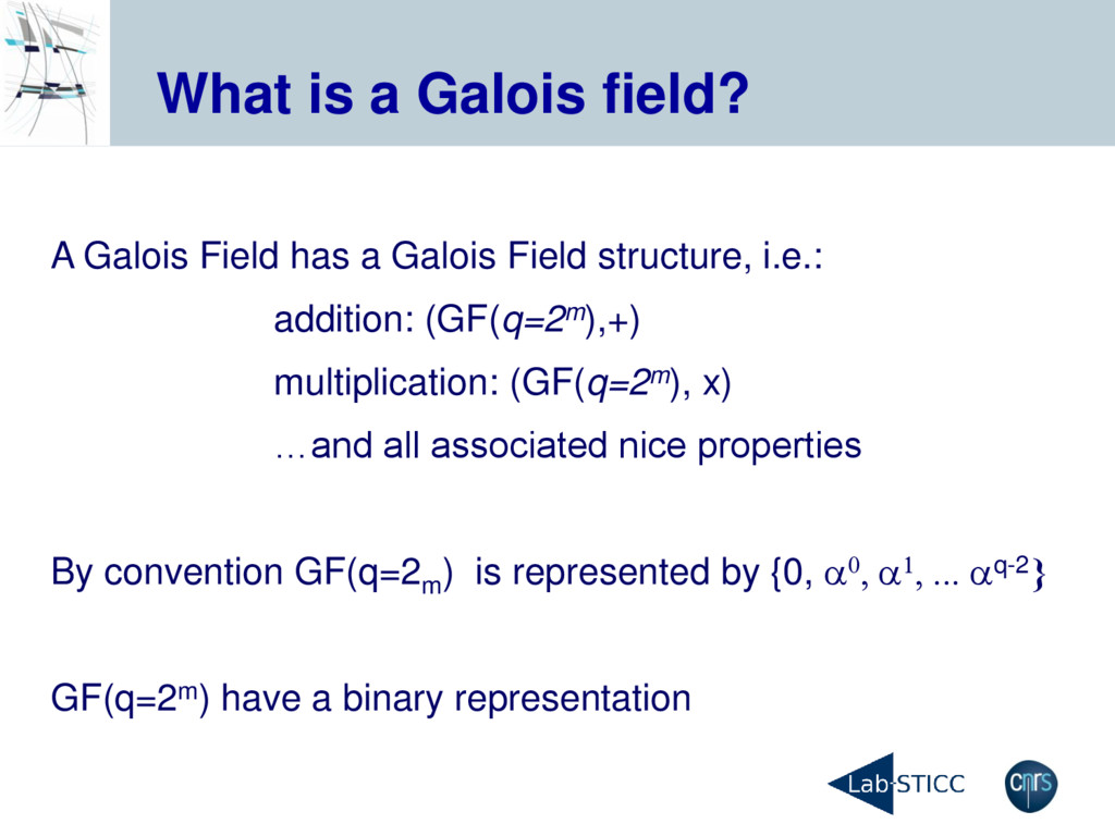
14. What is a Galois field? A Galois Field has a Galois Field structure, i.e.: addition: (GF(q=2m),+) multiplication: (GF(q=2m), x) …and all associated nice properties By convention GF(q=2m ) is represented by {0, a0, a1, ... aq-2} GF(q=2m) have a binary representation
15. Operation in GF(8) GF(8) bin 0 000 α0 100 α1 010 α2 001 α3 110 α4 011 α5 111 α6 101 Addition: x = (x1 x2 x3 ) and y = (y1 y2 y3 )  GF(8) x + y = (x1 x2 x3 ) XOR (y1 y2 y3 ) Example: α2+ α5= (001) XOR (111) = (110) =α3 Multiplication: 0  αi =0 αi  αj = α(i+j)mod(q-1) Example: α3  α5 = α(3+5)mod7 = α1 Binary representation:
16. OUTLINE 1) Introduction LDPC NB-LDPC Galois Field 2) Decoding NB-LDPC 3) What is the pro and cons of NB-LDPC?
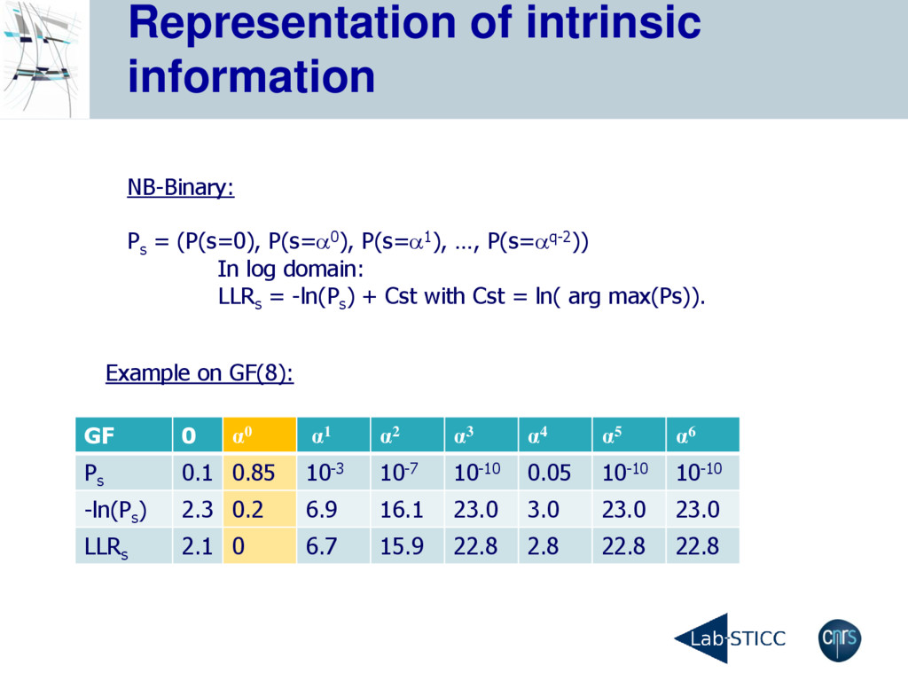
17. Representation of intrinsic information NB-LDPC Encoder Message of N ×m bits Modulation Channel Binary: (P(b=0), P(b=1))  LLR = ln(P(b=1)/P(b=0)) = ln(P(b=1))-ln(P(b=0)) NB-Binary: P s = (P(s=0), P(s=a0), P(s=a1), …, P(s=aq-2)) In log domain: LLR s = -ln(P s ) + Cst with Cst = ln( arg max(Ps)). Demodulation NB-LDPC decoder Message of K ×m bits LLR(s) Message of K × m bits
18. Representation of intrinsic information Example on GF(8): GF 0 α0 α1 α2 α3 α4 α5 α6 P s 0.1 0.85 10-3 10-7 10-10 0.05 10-10 10-10 -ln(P s ) 2.3 0.2 6.9 16.1 23.0 3.0 23.0 23.0 LLR s 2.1 0 6.7 15.9 22.8 2.8 22.8 22.8 NB-Binary: P s = (P(s=0), P(s=a0), P(s=a1), …, P(s=aq-2)) In log domain: LLR s = -ln(P s ) + Cst with Cst = ln( arg max(Ps)).
19. LLR computation for BPSK LLR(b j ) j=1..m ) ( )) ( )) ( ( ( ) ( 1 0 j j i q j i b LLR b HD j s LLR        a a Example: LLR(b 1 )=2 ; LLR(b 0 ) = -4 => Hard Decision : (1,0) => a1 LLR(s=0) = 2 0 = (0,0) LLR(s=a0) = 2 + 4 = 6 a0 = (0,1) LLR(s=a1) = 0 a1 = (1,0) LLR(s=a2) = 4 a2 = (1,1) NB-LDPC Encoder Message of N ×m bits BPSK Channel Demodulation NB-LDPC decoder Message of K ×m bits Message of K × m bits
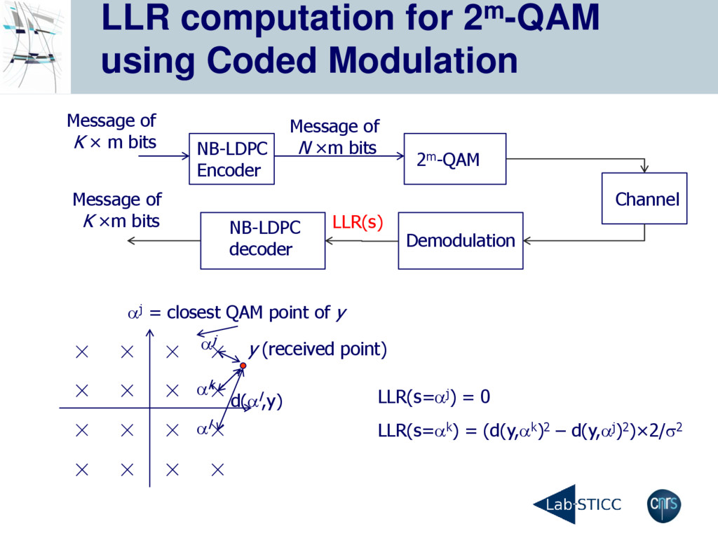
20. LLR computation for 2m-QAM using Coded Modulation y (received point) aj ak LLR(s=aj) = 0 LLR(s=ak) = (d(y,ak)2 – d(y,aj)2)×2/s2 aj = closest QAM point of y al d(al,y) NB-LDPC Encoder Message of N ×m bits 2m-QAM Channel Demodulation NB-LDPC decoder Message of K ×m bits LLR(s) Message of K × m bits
21. LLR computation for 2m-QAM using Bit-Interleaved Coded Modulation y (received point) d(al,y) P P1 ) ( )) ( )) ( ( ( ) ( 1 0 j j i q j i b LLR b HD j s LLR        a a 1000. 1010. 1001. 1011. 0010. 0000. 0011. 0001. 1101. 1111. 0111. 0101. 1100. 1110. 0110. 0100.                  1 1 0 0 ) ( ) ( log ) ( 1 0 j j GF x GF x j x p x p b LLR NB-LDPC Encoder 2m-QAM Channel Demodulation Binary LDPC decoder Message of K ×m bits LLR(s) Message of K × m bits Bit marginalization lead to loss of information
22. Variable node processing Variable node Intrinsic M c→v Mv→c = Adition term by term addition of I and Mc→v Then normalization. GF LLR 0 3 α0 17 α1 0 α2 9 GF LLR 0 8 α0 15 α1 7 α2 8 GF LLR 0 11 α0 32 α1 7 α2 17 Intrinsic M c→v M v→c + = Example in GF(4): GF LLR 0 4 α0 25 α1 0 α2 10 M v→c -
23. Edge processing Variable node The effect of edge multiplication is just a permutation of the LLR M v→m = (0, 13, 7, 14) x 1 a (0, 7, 14, 13)= M m→c  a1(0, a0, a1, a2) = (0, a1, a2, a0)
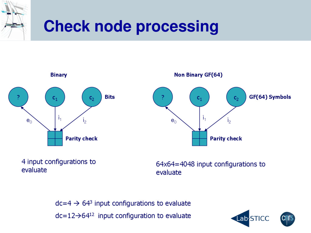
24. Check node processing GF(64) Symbols Parity check Parity check Bits ? c1 c2 i 2 i 1 e 0 ? c1 c2 i 2 i 1 e 0 Binary Non Binary GF(64) 4 input configurations to evaluate 64x64=4048 input configurations to evaluate dc=4  643 input configurations to evaluate dc=126412 input configuration to evaluate
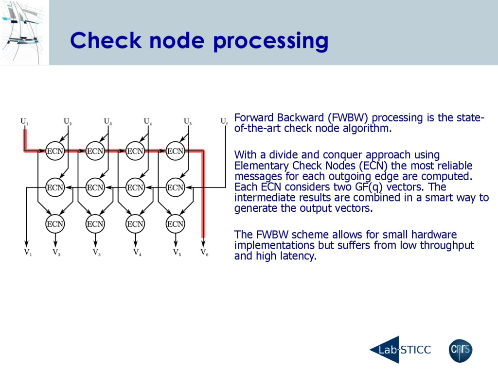
25. Check node processing Forward Backward (FWBW) processing is the state- of-the-art check node algorithm. With a divide and conquer approach using Elementary Check Nodes (ECN) the most reliable messages for each outgoing edge are computed. Each ECN considers two GF(q) vectors. The intermediate results are combined in a smart way to generate the output vectors. The FWBW scheme allows for small hardware implementations but suffers from low throughput and high latency.
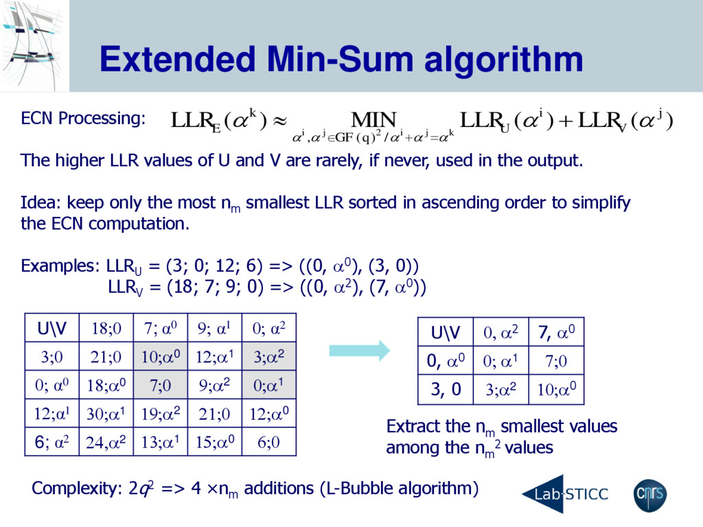
26. Extended Min-Sum algorithm ECN Processing: The higher LLR values of U and V are rarely, if never, used in the output. Idea: keep only the most n m smallest LLR sorted in ascending order to simplify the ECN computation. Examples: LLR U = (3; 0; 12; 6) => ((0, a0), (3, 0)) LLR V = (18; 7; 9; 0) => ((0, a2), (7, a0)) ) ( ) ( ) ( / ) ( , 2 j V i U q GF k E LLR LLR MIN LLR k j i j i a a a a a a a a      U\V 18;0 7; α0 9; α1 0; α2 3;0 21;0 10;a0 12;a1 3;a2 0; α0 18;a0 7;0 9;a2 0;a1 12;α1 30;a1 19;a2 21;0 12;a0 6; α2 24,a2 13;a1 15;a0 6;0 U\V 0, a2 7, a0 0, a0 0; a1 7;0 3, 0 3;a2 10;a0 Extract the n m smallest values among the n m 2 values Complexity: 2q2 => 4 ×n m additions (L-Bubble algorithm)
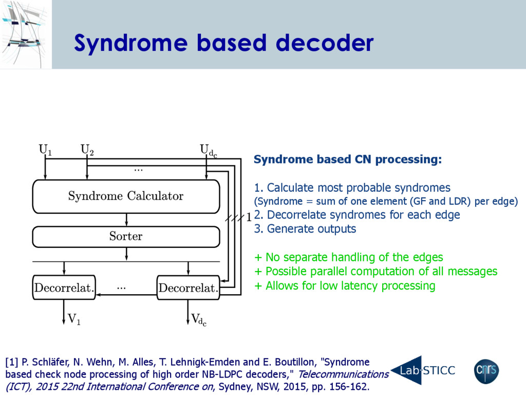
27. Syndrome based decoder Syndrome based CN processing: 1. Calculate most probable syndromes (Syndrome = sum of one element (GF and LDR) per edge) 2. Decorrelate syndromes for each edge 3. Generate outputs + No separate handling of the edges + Possible parallel computation of all messages + Allows for low latency processing [1] P. Schläfer, N. Wehn, M. Alles, T. Lehnigk-Emden and E. Boutillon, "Syndrome based check node processing of high order NB-LDPC decoders," Telecommunications (ICT), 2015 22nd International Conference on, Sydney, NSW, 2015, pp. 156-162.
28. OUTLINE 1) Introduction LDPC NB-LDPC Galois Field 2) Decoding NB-LDPC 3) What are the pro and cons of NB-LDPC ?
29. Cons - Changing from LDPC to NB-LDPC is a revolution (no more compatibility). -Complexity
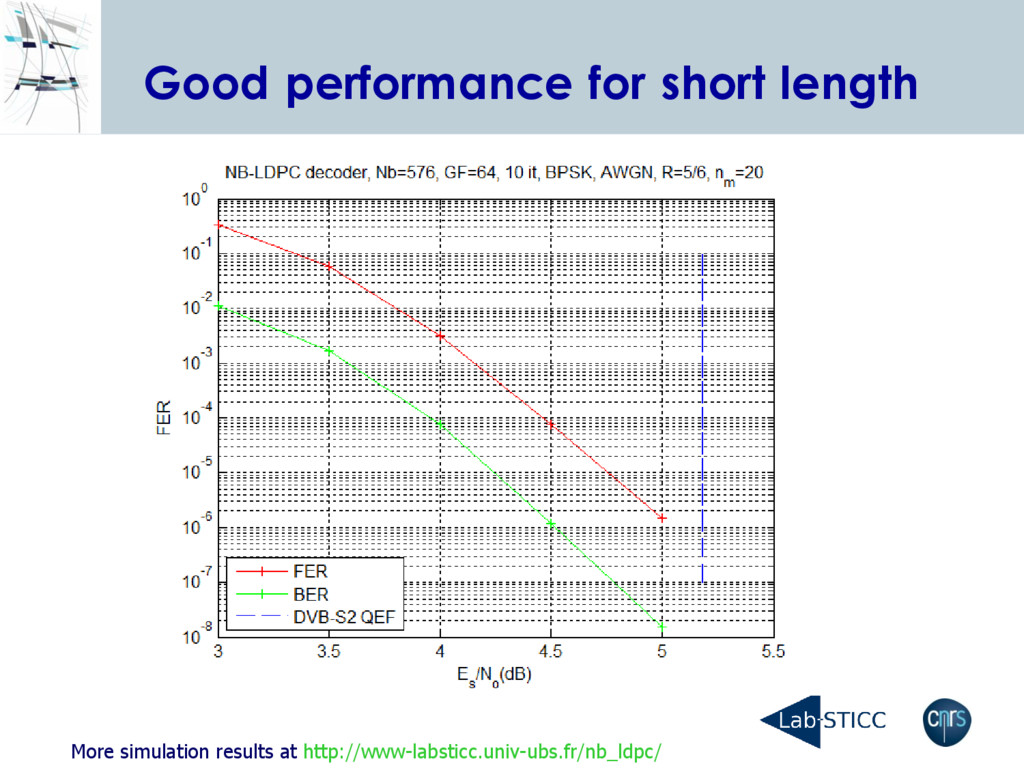
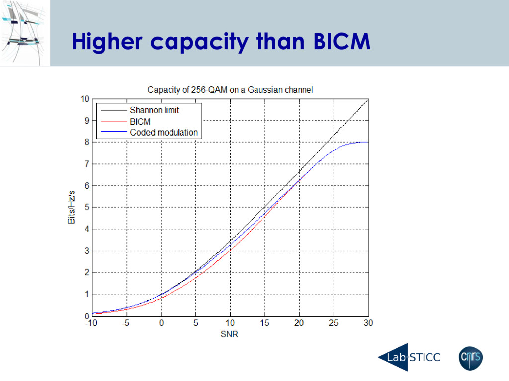
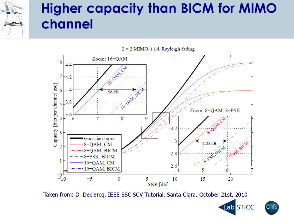
30. Pros… - Under BP decoding, NB-LDPC has significant better performance than LDPC for low code size and low code rate. -Low error floor -No need of bit marginalization during the demodulation (high spectral efficiency). - Higher mutual information of Coded Modulation VS BICM (in SISO, SIMO, MIMO, … channel).
31. Good performance for short length More simulation results at http://www-labsticc.univ-ubs.fr/nb_ldpc/
32. Higher capacity than BICM
33. Higher capacity than BICM for MIMO channel Taken from: D. Declercq, IEEE SSC SCV Tutorial, Santa Clara, October 21st, 2010
34. Conclusion NB-LDPC is not yet a mature technology : great potential improvement. - Under BP decoding, NB-LDPC has significant better performance than LDPC for low code size and low code rate. -No need of bit marginalization during the demodulation (high spectral efficiency). - Higher mutual information of Coded Modulation VS BICM (in SISO, SIMO, MIMO, … channel).
35. Conclusion  Thank you for your attention  Questions are welcome 35