Hamed Ahmadi - Learning, prediction and selection algorithms for opportunistic spectrum access

Transcript

1. Learning, prediction and selection algorithms for opportunistic spectrum access Hamed Ahmadi Research Fellow, CTVR, Trinity College Dublin TRINITY COLLEGE DUBLIN
2. Future Cellular, Wireless, Next Generation Broadband & IoT
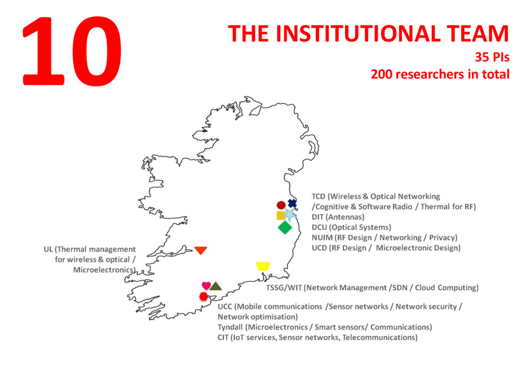
3. CONNECT is a one stop shop for all things to do with future networks and communications in Ireland. IoT Wireless Cellular Fixed hardware, software, infrastructure, architecture, management, applications, services …
4. THE INSTITUTIONAL TEAM 35 PIs 200 researchers in total 10
6. THE INDUSTRY TEAM 35+
7. Learning, prediction and selection algorithms for opportunistic spectrum access
8. Opportunistic spectrum access
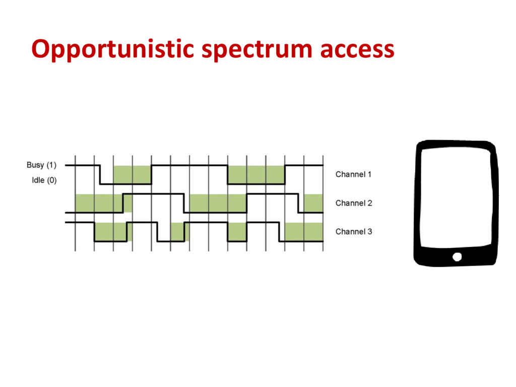
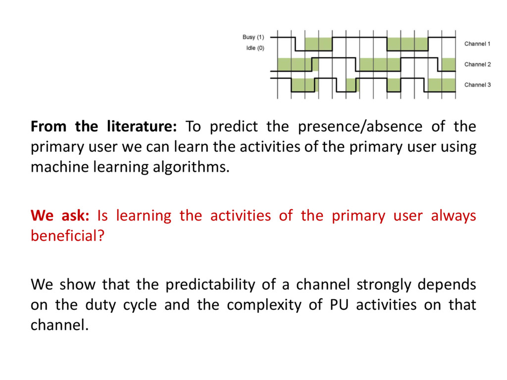
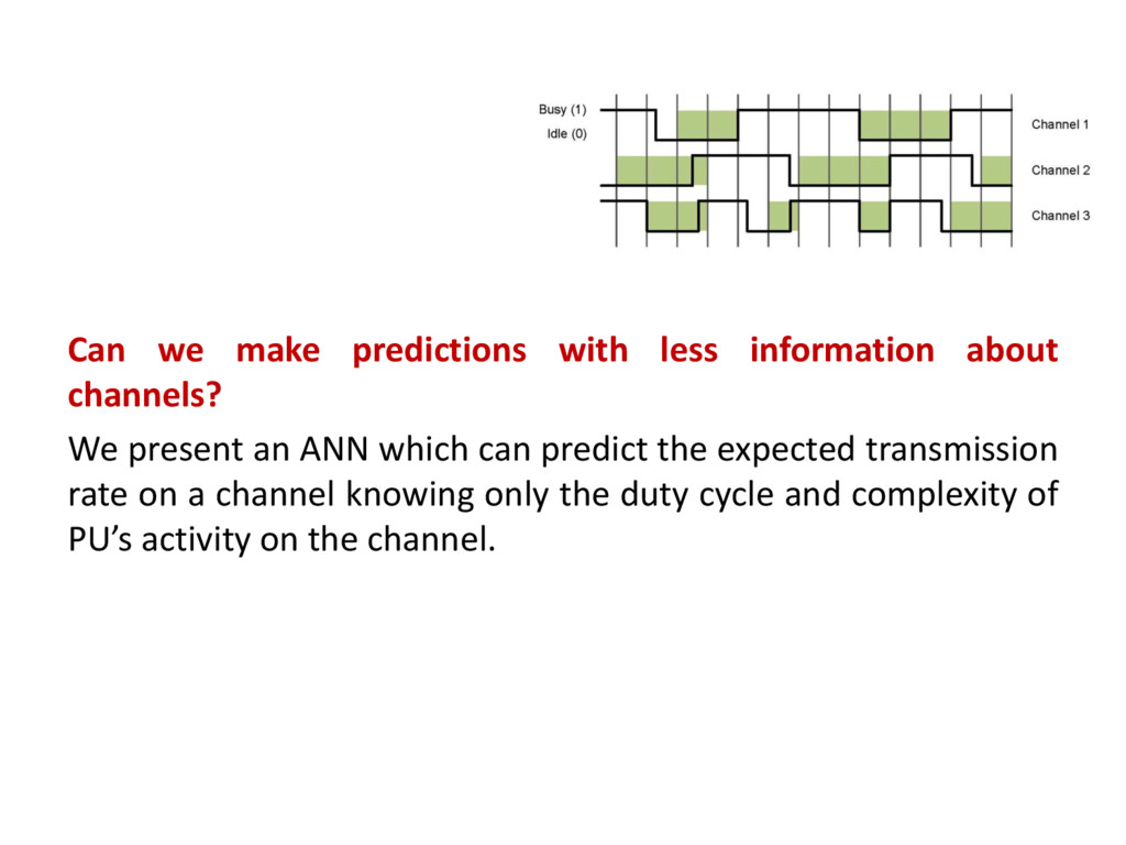
9. From the literature: To predict the presence/absence of the primary user we can learn the activities of the primary user using machine learning algorithms. We ask: Is learning the activities of the primary user always beneficial? We show that the predictability of a channel strongly depends on the duty cycle and the complexity of PU activities on that channel.
10. Can we make predictions with less information about channels? We present an ANN which can predict the expected transmission rate on a channel knowing only the duty cycle and complexity of PU’s activity on the channel.
11. Do we need to observe all the channels? With a greedy algorithm we select a subset of channels to observe and compare its performance with the performance of the system when observing all channels.
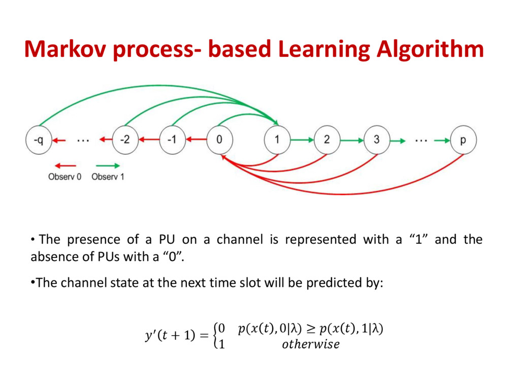
12. Markov process- based Learning Algorithm • The presence of a PU on a channel is represented with a “1” and the absence of PUs with a “0”. •The channel state at the next time slot will be predicted by: ′ + 1 = 0 ( , 0|λ) ≥ ( , 1|λ) 1 ℎ
13. Duty cycle and Lempel-Ziv complexity • A spectrum occupancy sequence can be characterized in terms of the observed DC and the complexity of the PU activity. • Each channel is the realization of a 2-state first order Markov chain (MC). • For an ergodic source the Lempel-Ziv complexity equals the entropy rate of the source, which for a Markov chain X is given by: ℎ = − log
14. Impact of LZ and DC on the prediction accuracy • We considered 5 possible δ0 values in the range 0.5, … , 0.9. For each of these values, we considered 5 transition probability matrices, each corresponding to a different value of entropy rate. • At each point K = 3 channels. • Pf is the probability of at least one free channel existing.
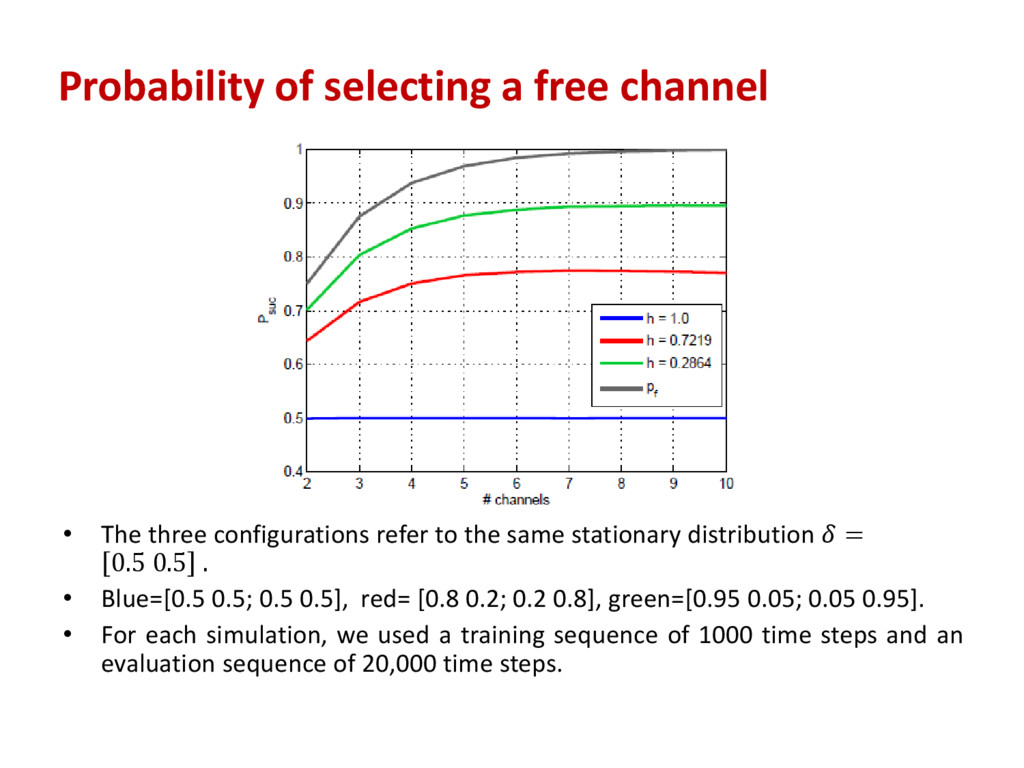
15. Probability of selecting a free channel • The three configurations refer to the same stationary distribution = 0.5 0.5 . • Blue=[0.5 0.5; 0.5 0.5], red= [0.8 0.2; 0.2 0.8], green=[0.95 0.05; 0.05 0.95]. • For each simulation, we used a training sequence of 1000 time steps and an evaluation sequence of 20,000 time steps.
16. Reducing the number of channels Here 3 channels are characterized by DC = 0.6 (low, medium and high complexity) and the other 3 channels correspond to DC = 0.5 (low, medium and high complexity).
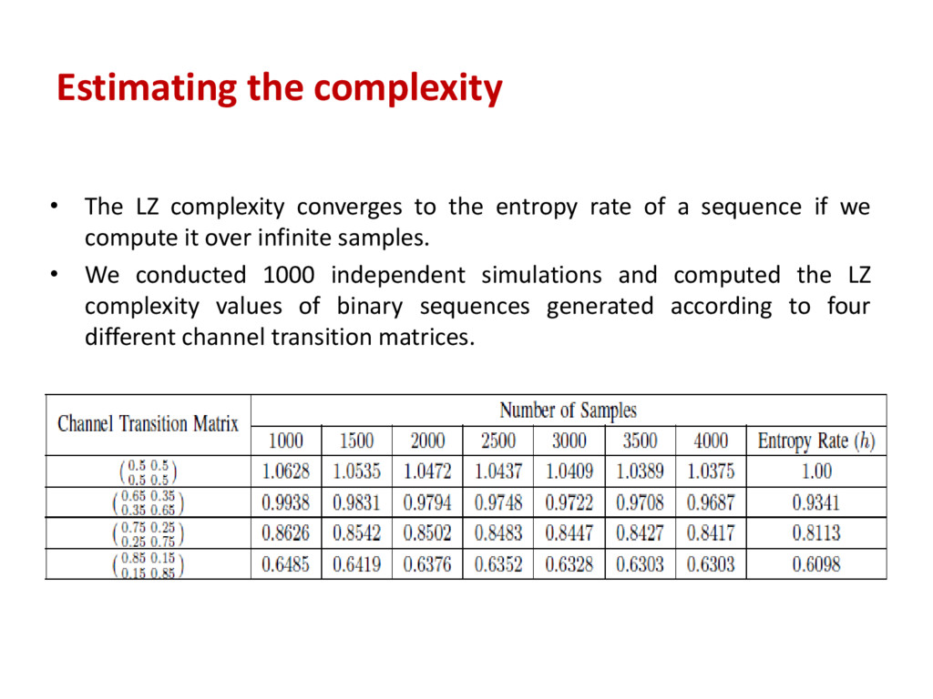
17. Estimating the complexity • The LZ complexity converges to the entropy rate of a sequence if we compute it over infinite samples. • We conducted 1000 independent simulations and computed the LZ complexity values of binary sequences generated according to four different channel transition matrices.
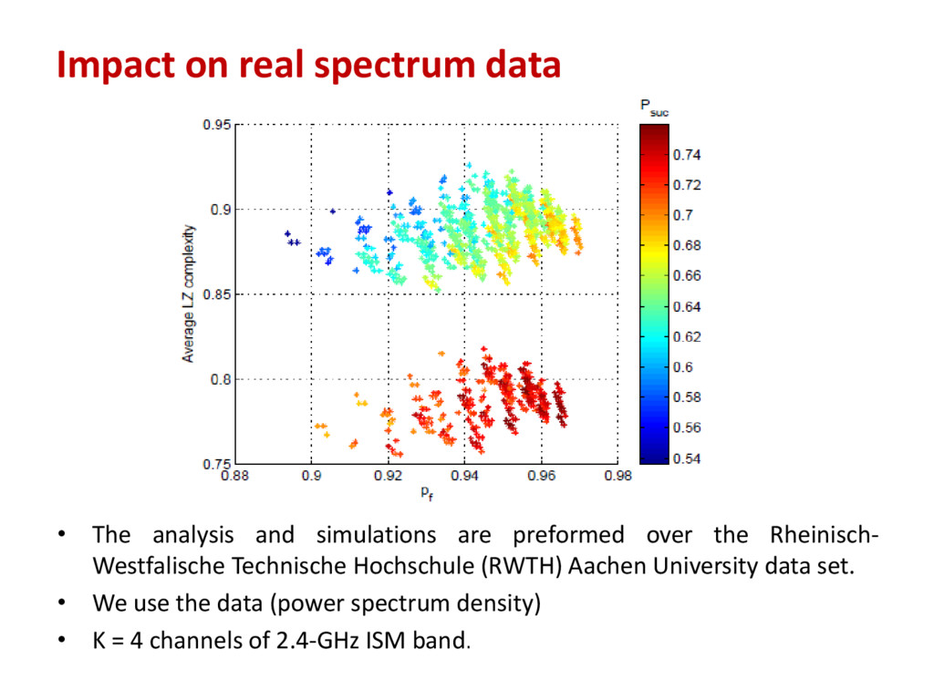
18. • The analysis and simulations are preformed over the Rheinisch- Westfalische Technische Hochschule (RWTH) Aachen University data set. • We use the data (power spectrum density) • K = 4 channels of 2.4-GHz ISM band Impact on real spectrum data
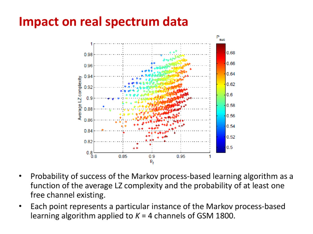
19. • Probability of success of the Markov process-based learning algorithm as a function of the average LZ complexity and the probability of at least one free channel existing. • Each point represents a particular instance of the Markov process-based learning algorithm applied to K = 4 channels of GSM 1800. Impact on real spectrum data
20. There are many more channels to observe in reality!!!
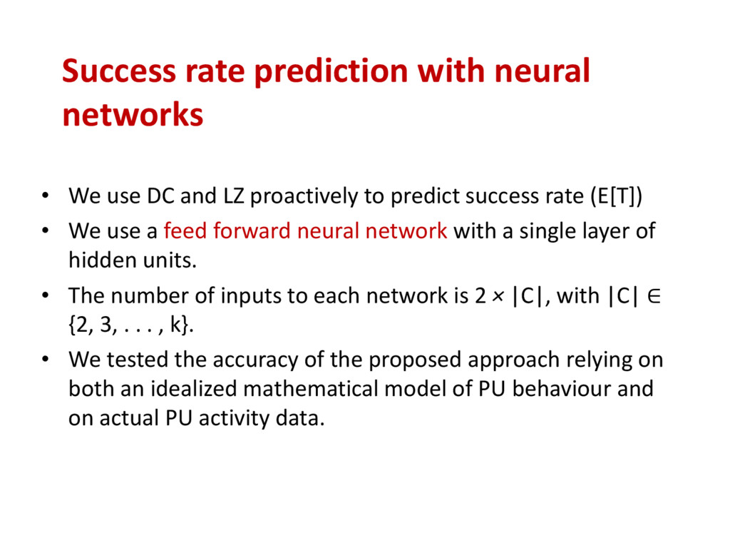
21. • We use DC and LZ proactively to predict success rate (E[T]) • We use a feed forward neural network with a single layer of hidden units. • The number of inputs to each network is 2 × |C|, with |C| ∈ {2, 3, . . . , k}. • We tested the accuracy of the proposed approach relying on both an idealized mathematical model of PU behaviour and on actual PU activity data. Success rate prediction with neural networks
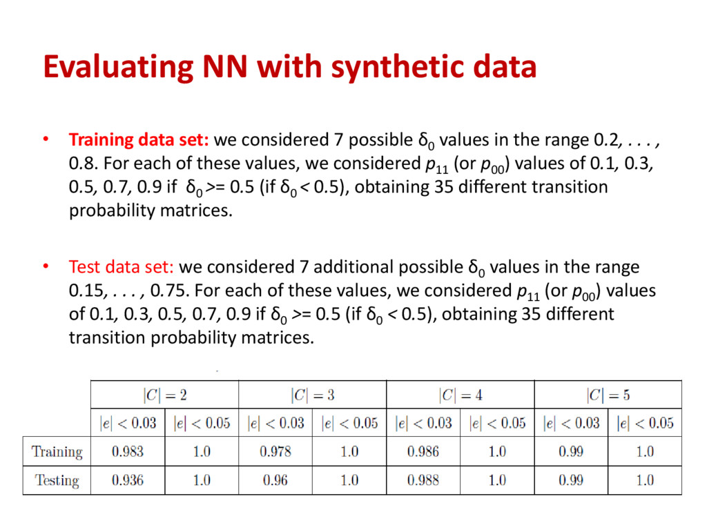
22. Evaluating NN with synthetic data • Training data set: we considered 7 possible δ0 values in the range 0.2, . . . , 0.8. For each of these values, we considered p11 (or p00 ) values of 0.1, 0.3, 0.5, 0.7, 0.9 if δ0 >= 0.5 (if δ0 < 0.5), obtaining 35 different transition probability matrices. • Test data set: we considered 7 additional possible δ0 values in the range 0.15, . . . , 0.75. For each of these values, we considered p11 (or p00 ) values of 0.1, 0.3, 0.5, 0.7, 0.9 if δ0 >= 0.5 (if δ0 < 0.5), obtaining 35 different transition probability matrices.
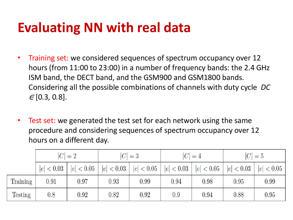
23. Evaluating NN with real data • Training set: we considered sequences of spectrum occupancy over 12 hours (from 11:00 to 23:00) in a number of frequency bands: the 2.4 GHz ISM band, the DECT band, and the GSM900 and GSM1800 bands. Considering all the possible combinations of channels with duty cycle DC ∈ [0.3, 0.8]. • Test set: we generated the test set for each network using the same procedure and considering sequences of spectrum occupancy over 12 hours on a different day.
24. The problem is not totally solved yet! We cannot observe all channels!
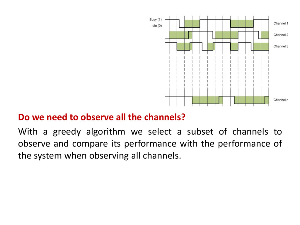
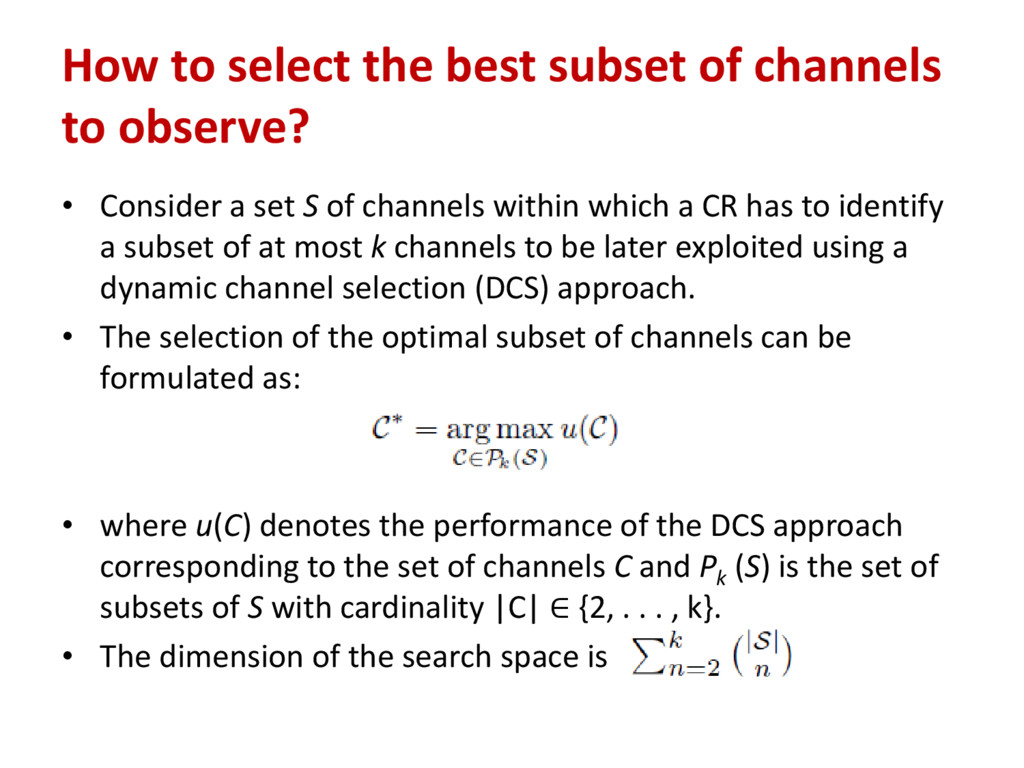
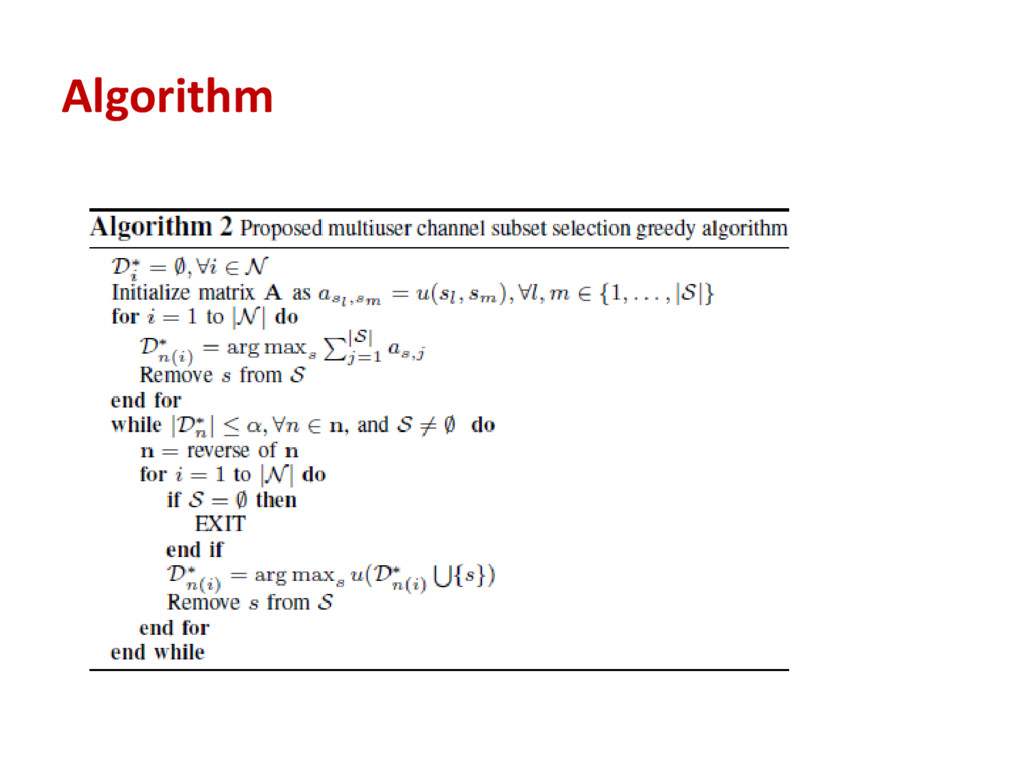
25. How to select the best subset of channels to observe? • Consider a set S of channels within which a CR has to identify a subset of at most k channels to be later exploited using a dynamic channel selection (DCS) approach. • The selection of the optimal subset of channels can be formulated as: • where u(C) denotes the performance of the DCS approach corresponding to the set of channels C and Pk (S) is the set of subsets of S with cardinality |C| ∈ {2, . . . , k}. • The dimension of the search space is
26. Channel Subset selection algorithm • To reduce the search space we propose a greedy algorithm
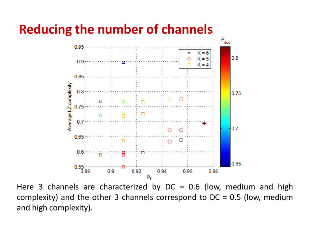
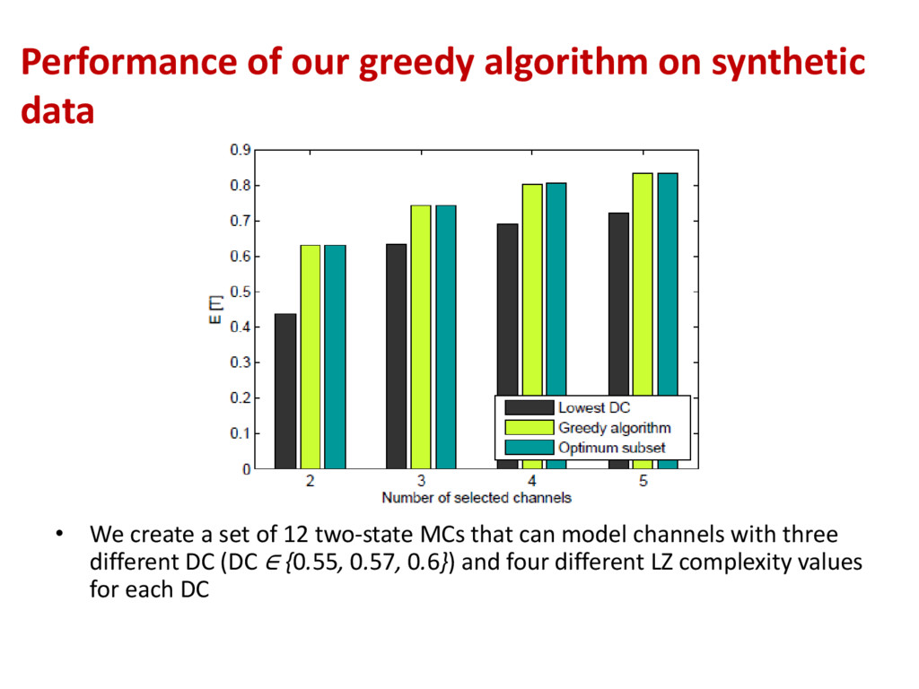
27. Performance of our greedy algorithm on synthetic data • We create a set of 12 two-state MCs that can model channels with three different DC (DC ∈ {0.55, 0.57, 0.6}) and four different LZ complexity values for each DC
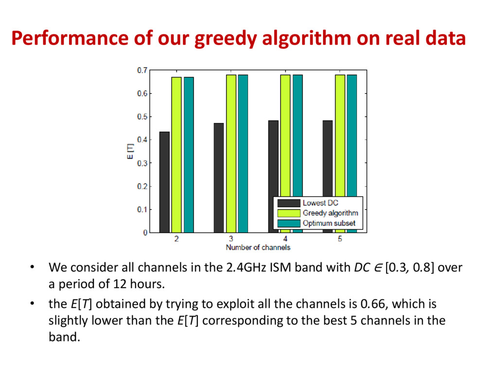
28. Performance of our greedy algorithm on real data • We consider all channels in the 2.4GHz ISM band with DC ∈ [0.3, 0.8] over a period of 12 hours. • the E[T] obtained by trying to exploit all the channels is 0.66, which is slightly lower than the E[T] corresponding to the best 5 channels in the band.
29. NN-based Greedy algorithm • 2.4GHz ISM band: the difference in performance between the E[T] corresponding to the optimum subset and the E[T] of NN- based exhaustive search(e1) and NN-based greedy algorithm (e2).
30. Selecting fungible channel sets for multiple users
31. Bundling of channels • Assigning fungible channel sets to different CRs 31
32. Low-High complexity The average difference between the performance of the Markov process-based learning algorithm on the optimum subsets and the subsets of channels with Lowest DC (LDC). We consider 3 users, 10 channels with high LZ and base-DC, and 10 channels with low LZ and DC=base-DC+Δ.
33. Algorithm
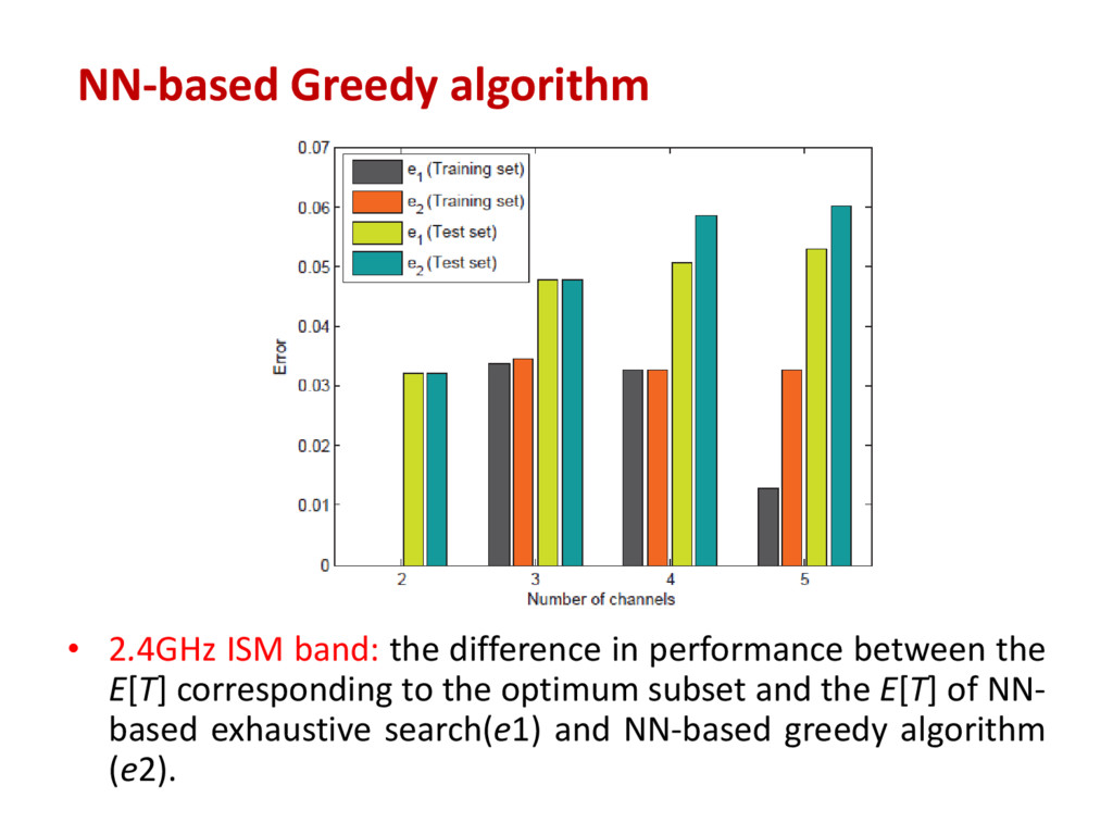
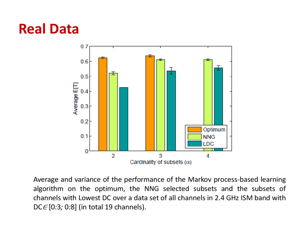
34. Real Data Average and variance of the performance of the Markov process-based learning algorithm on the optimum, the NNG selected subsets and the subsets of channels with Lowest DC over a data set of all channels in 2.4 GHz ISM band with DC∈ [0:3; 0:8] (in total 19 channels).
35. What if the channel statistics significantly change?
36. Summary • What we did is
37. Summary • What we did is • And what we are going to do is
38. Carrier Aggregation as a Repeated Game: Learning Algorithms for Efficient Convergence to a Nash Equilibrium
39. “In Game of thrones you either WIN or you DIE” Cersei Lannister
40. “In Game of thrones you either WIN or you DIE” Cersei Lannister In Game theory we study the mathematical models of conflict and cooperation between intelligent rational decision-makers
41. Motivation • Extension of current static CA to dynamic CA has been explored recently • Dynamic CA is possible in a distributed manner • Few works allow each network to aggregate non-contiguous channels in multiple frequency bands • Effect of out-of-channel (OOC) interference in adjacent frequency channels is not considered in existing works Ahmadi H, Macaluso I, DaSilva L.A, “Carrier aggregation as a repeated game: learning algorithms for efficient convergence to a Nash equilibrium”, Accepted in IEEE Globcom’13.
42. What we do • Model the preference for contiguous channels aggregation • Assign a higher cost to the inter-band CA • Model the problem of dynamic CA as a non-cooperative game • Propose learning algorithms that converge to a pure NE within a reasonable number of iterations under the conditions of incomplete and imperfect information
43. Intra-band and inter-band CA nbands(a) is the number of bands that a node accesses when selecting action a
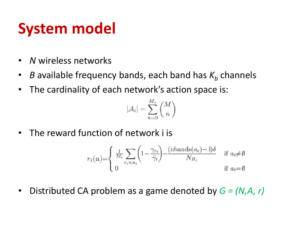
44. System model • N wireless networks • B available frequency bands, each band has Kb channels • The cardinality of each network’s action space is: • The reward function of network i is • Distributed CA problem as a game denoted by G = (N,A, r)
45. ITEL-BA
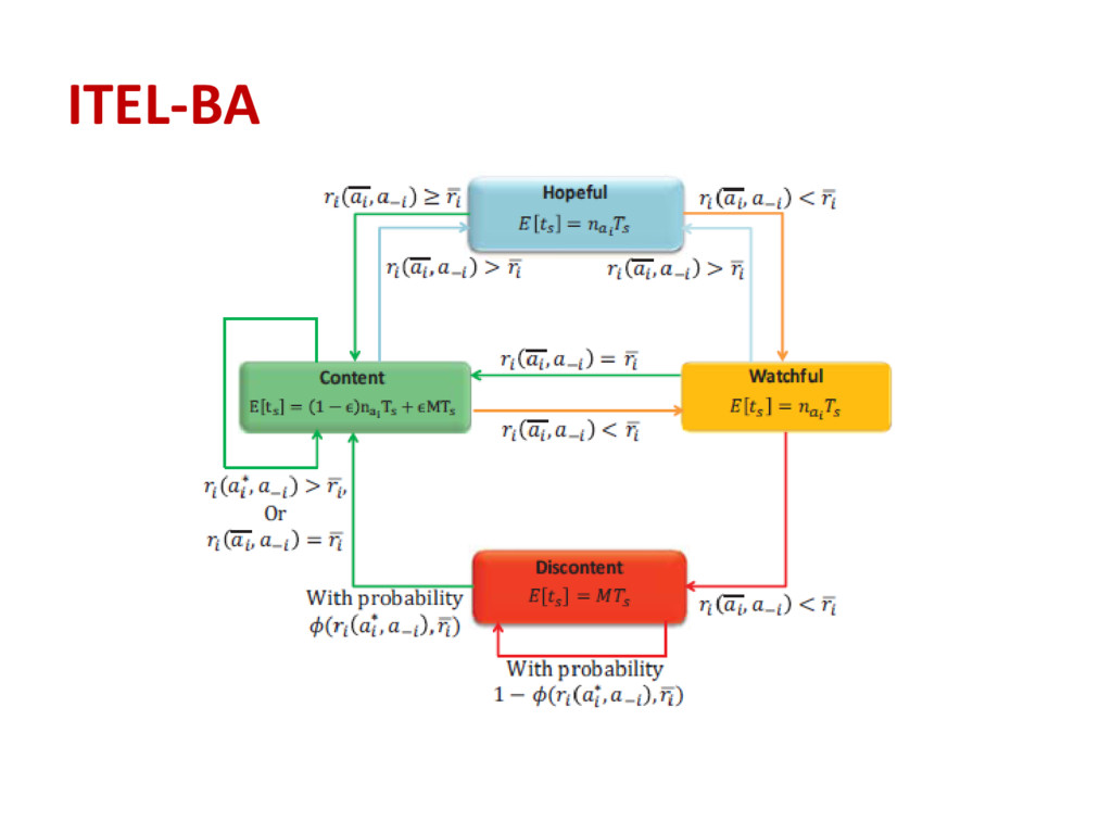
46. ITEL-BA with imperfect information • To deal with noisy feedback/sensing, each player computes the received and hypothetical payoffs and then updates () using an n-sample weighted moving average • In ITEL-BAWII, when a player experiments with new actions either in content or discontent mood, she will select the action that maximizes the average estimated payoff () • The expected sensing time is TsM for all the states
47. Results Convergence probability of ITEL-BA to an NE for different scenarios
48. Results Convergence probability of ITEL-BA and ITEL-BAWII when the observations are not perfect
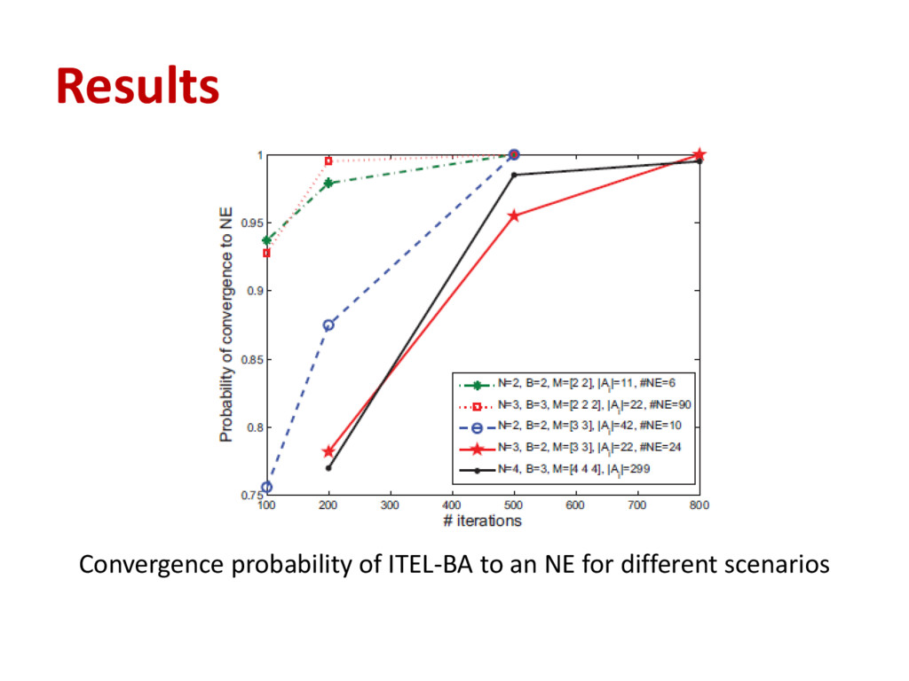
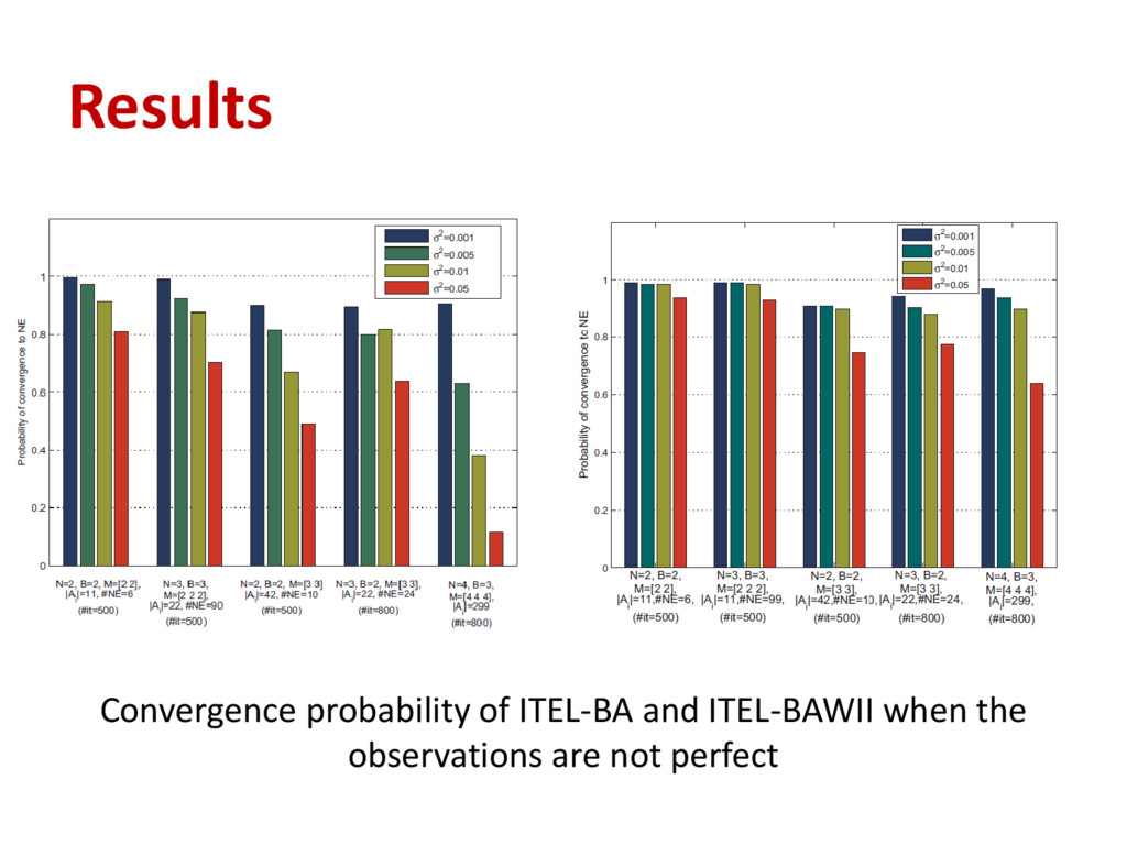
49. Conclusions • We modelled CA problem of autonomous networks operating in shared spectrum as a repeated game • We proposed learning algorithms that efficiently converge to an NE without the need for complete or even perfect information • Our results show that the algorithm, which effectively converges to an NE with incomplete information (ITEL-BA), is not efficient in the case of imperfect information • Our algorithm that effectively deals with imperfect and incomplete information (ITELBAWII) requires additional sensing and computational resources
50. Thank you Questions?