(GTAS, in Spanish) is part of the Communications Engineering Department of the University of Cantabria. It is located at the E.T.S.I. Industriales y Telecomunicaciones, Avda Los Castros s/n. Santander 39005, SPAIN. The Advanced Signal Processing Group http://gtas.unican.es
communication links. • CSI (Channel State Information) estimation techniques, synchronization, detection techniques,... • Capacity analysis of MIMO links. • Development of hardware MIMO testbeds and performance evaluation. •Machine-learning techniques and their application to communications. • Kernel methods, neural networks and adaptive information processing systems. • Multivariate statistical techniques: PCA, CCA and ICA. • Nonlinear modeling and nonlinear dynamical systems (chaos).
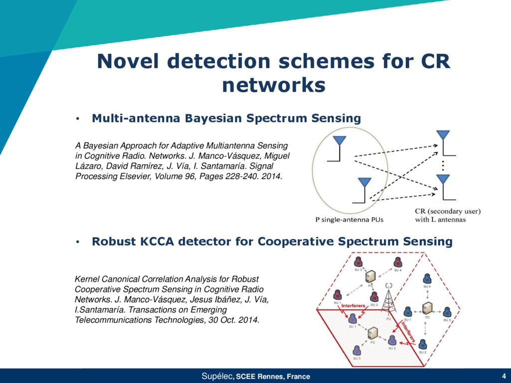
• Robust KCCA detector for Cooperative Spectrum Sensing Novel detection schemes for CR networks A Bayesian Approach for Adaptive Multiantenna Sensing in Cognitive Radio. Networks. J. Manco-Vásquez, Miguel Lázaro, David Ramírez, J. Vía, I. Santamaría. Signal Processing Elsevier, Volume 96, Pages 228-240. 2014. Kernel Canonical Correlation Analysis for Robust Cooperative Spectrum Sensing in Cognitive Radio Networks. J. Manco-Vásquez, Jesus Ibáñez, J. Vía, I.Santamaría. Transactions on Emerging Telecommunications Technologies, 30 Oct. 2014.
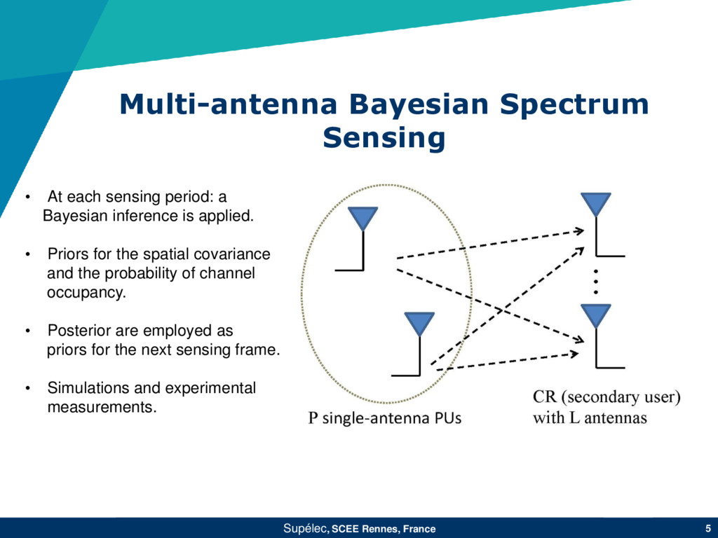
At each sensing period: a Bayesian inference is applied. • Priors for the spatial covariance and the probability of channel occupancy. • Posterior are employed as priors for the next sensing frame. • Simulations and experimental measurements.
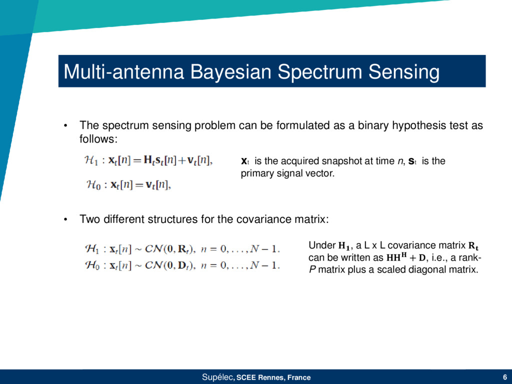
Two different structures for the covariance matrix: • The spectrum sensing problem can be formulated as a binary hypothesis test as follows: xt is the acquired snapshot at time n, st is the primary signal vector. Under , a L x L covariance matrix can be written as + , i.e., a rank- P matrix plus a scaled diagonal matrix.
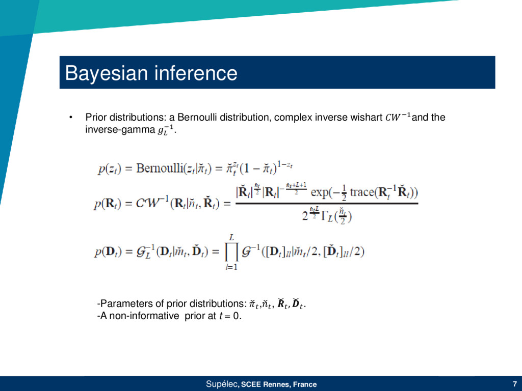
a Bernoulli distribution, complex inverse wishart −1and the inverse-gamma −1. -Parameters of prior distributions: , , , . -A non-informative prior at t = 0.
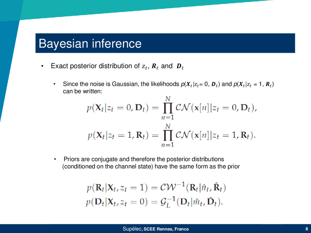
noise is Gaussian, the likelihoods p(|= 0, ) and p(| = 1, ) can be written: • Priors are conjugate and therefore the posterior distributions (conditioned on the channel state) have the same form as the prior • Exact posterior distribution of , and
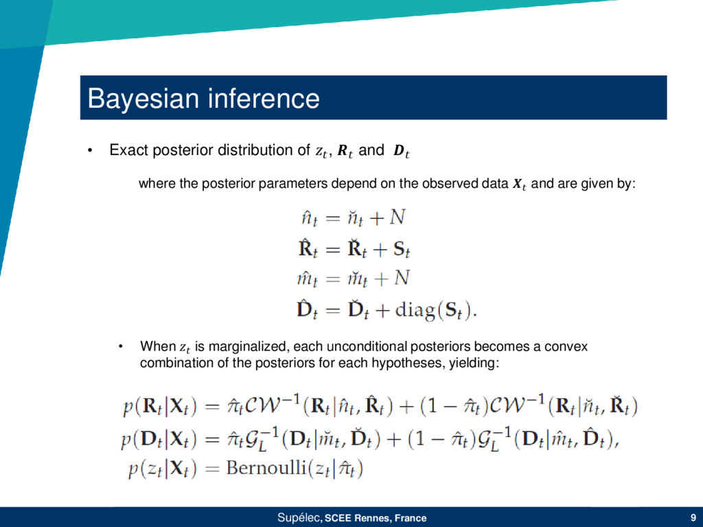
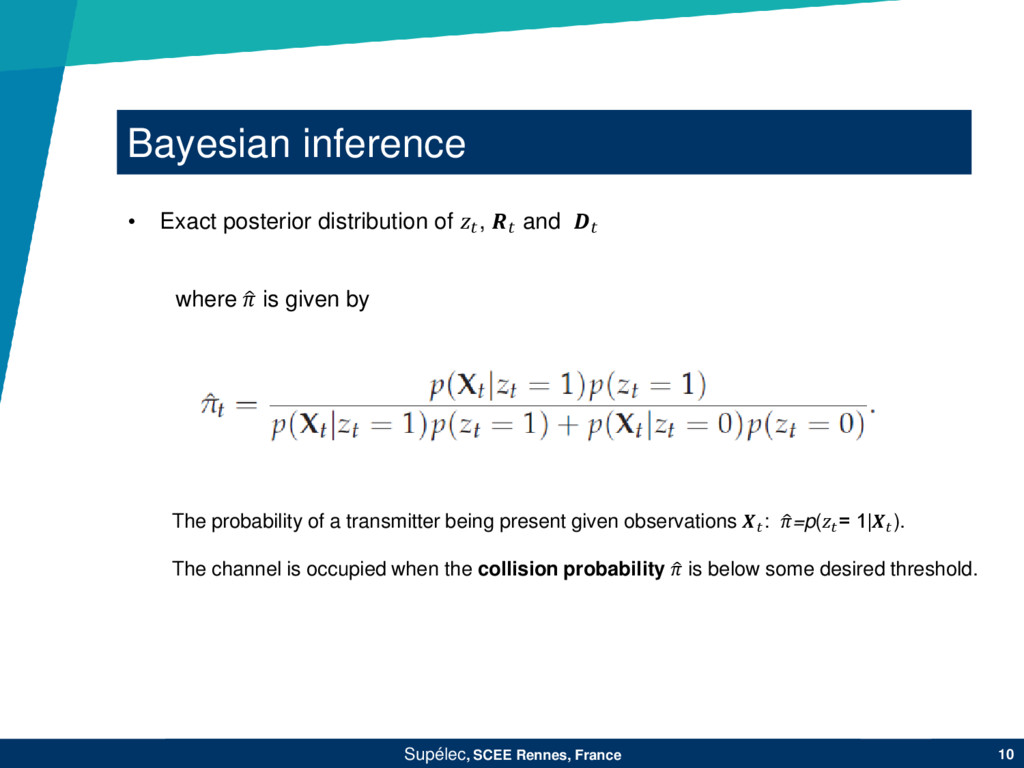
parameters depend on the observed data and are given by: • When is marginalized, each unconditional posteriors becomes a convex combination of the posteriors for each hypotheses, yielding: • Exact posterior distribution of , and
a transmitter being present given observations : =p( = 1|). The channel is occupied when the collision probability is below some desired threshold. where is given by • Exact posterior distribution of , and
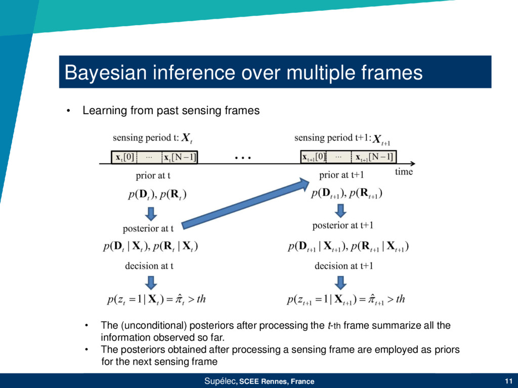
• The (unconditional) posteriors after processing the t-th frame summarize all the information observed so far. • The posteriors obtained after processing a sensing frame are employed as priors for the next sensing frame • Learning from past sensing frames
• Problem: The posterior distribution are convex combination of the posterior under each hypotheses • Thresholding-based approximation • Kullback-Leibler approximation Priors can be obtained by truncanting to either 0 or 1 whichever it is closer. A more rigororus approach is given by minimizing the KL distance
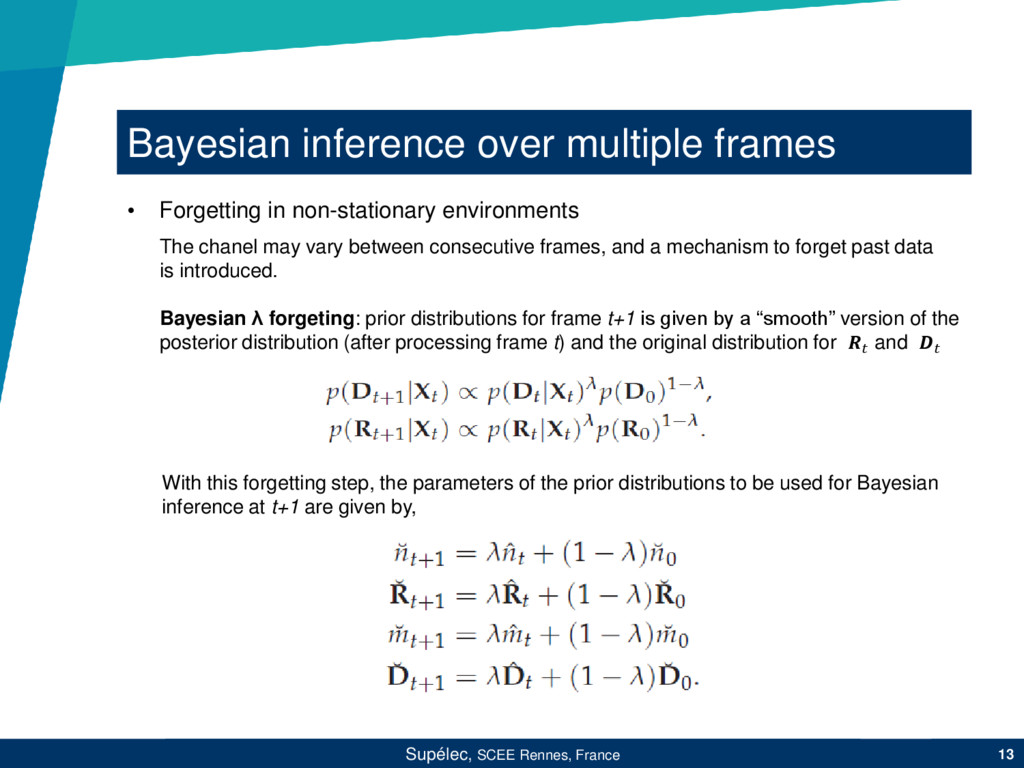
• Forgetting in non-stationary environments The chanel may vary between consecutive frames, and a mechanism to forget past data is introduced. Bayesian λ forgeting: prior distributions for frame t+1 is given by a “smooth” version of the posterior distribution (after processing frame t) and the original distribution for and With this forgetting step, the parameters of the prior distributions to be used for Bayesian inference at t+1 are given by,
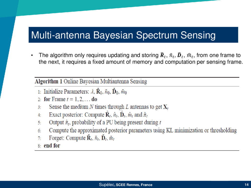
The algorithm only requires updating and storing , , , , from one frame to the next, it requires a fixed amount of memory and computation per sensing frame.
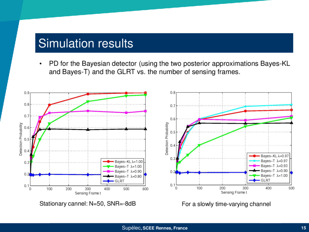
SNR=-8dB For a slowly time-varying channel • PD for the Bayesian detector (using the two posterior approximations Bayes-KL and Bayes-T) and the GLRT vs. the number of sensing frames.
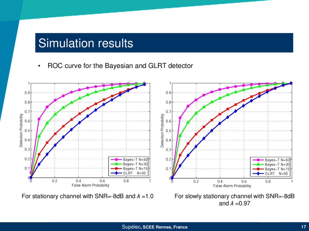
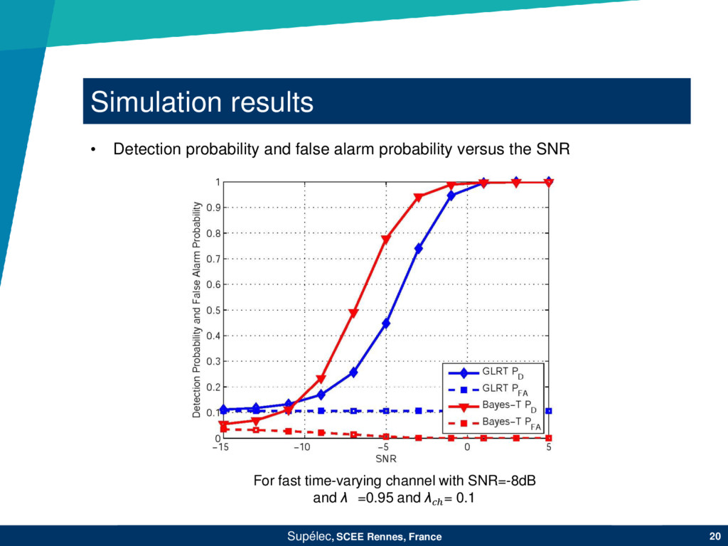
with SNR=-8dB λ=1.0, and λℎ=1 For slowly stationary channel with SNR=-8dB, λ =0.97,λℎ= 0.95 • Detection probability and false alarm probability versus SNR
with XCVR2450 daughterboard, two-antenna cognitive receiver compose of two N210 boards connected through a MIMO cable Laboratory equipment: signal generators, oscilloscopes, spectrum analyzers
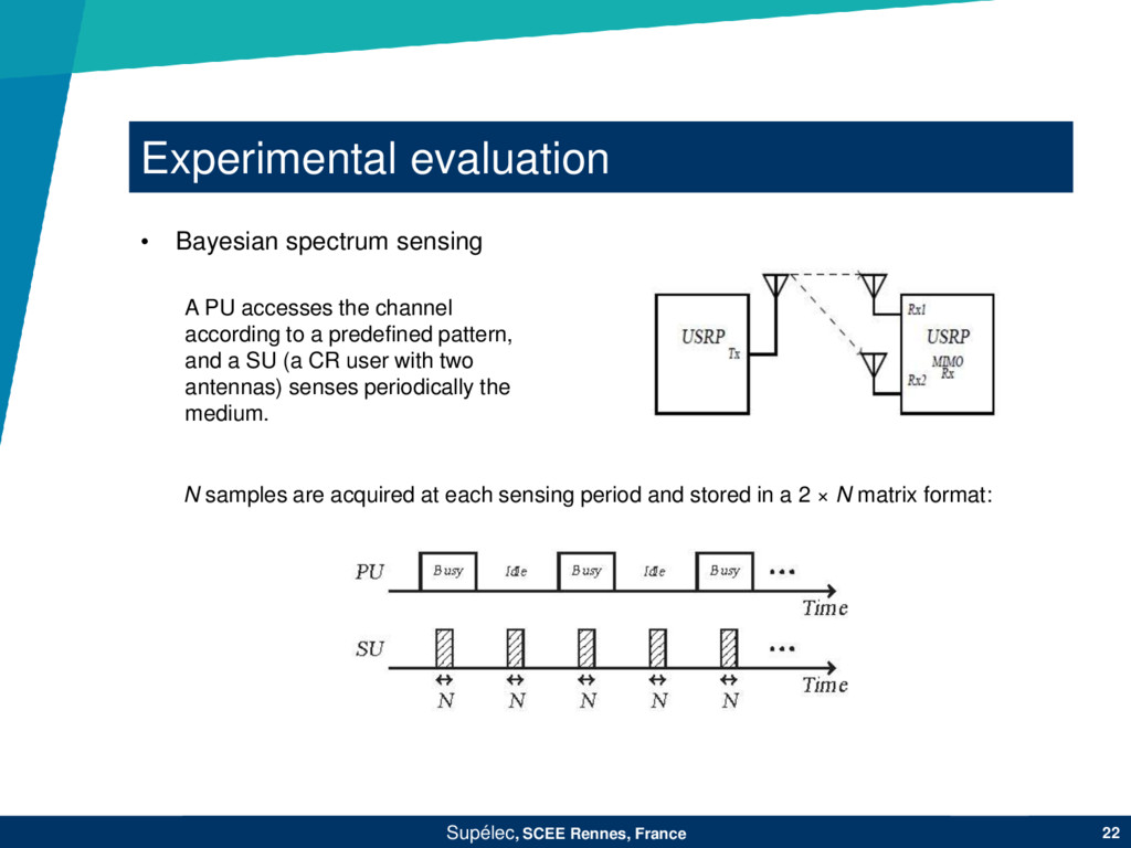
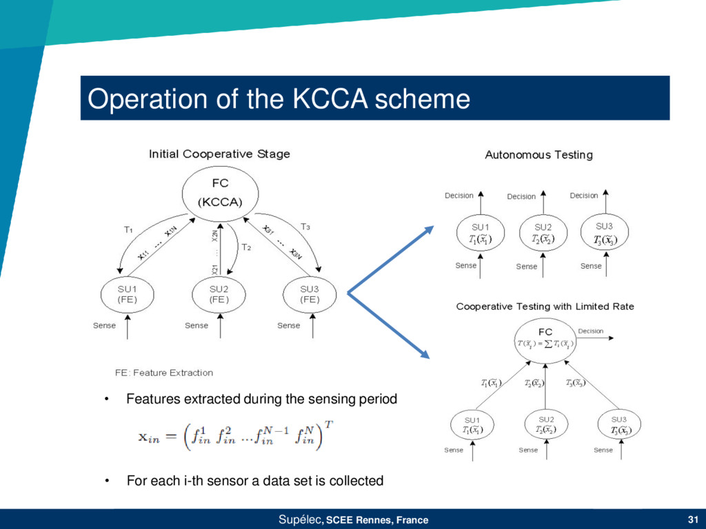
sensing A PU accesses the channel according to a predefined pattern, and a SU (a CR user with two antennas) senses periodically the medium. N samples are acquired at each sensing period and stored in a 2 × N matrix format:
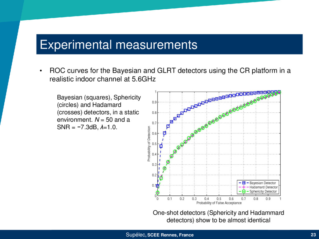
for the Bayesian and GLRT detectors using the CR platform in a realistic indoor channel at 5.6GHz One-shot detectors (Sphericity and Hadammard detectors) show to be almost identical Bayesian (squares), Sphericity (circles) and Hadamard (crosses) detectors, in a static environment. N = 50 and a SNR = −7.3dB, λ=1.0.
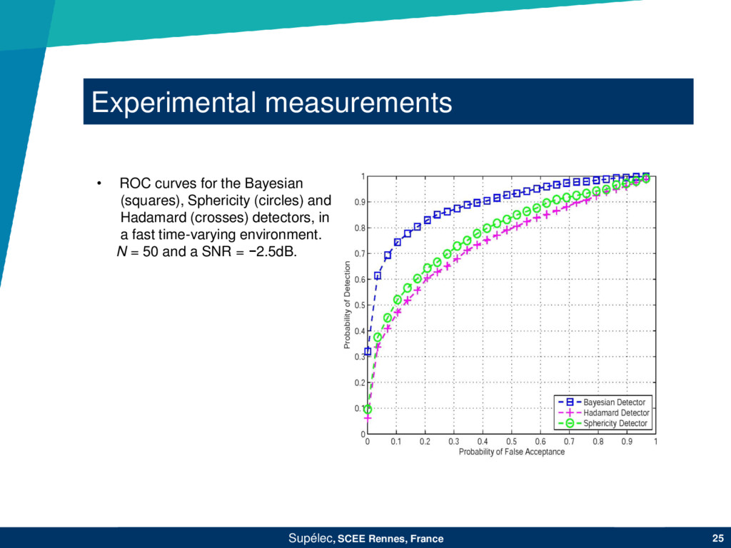
challenging scenario: the experimental evaluation in a non-stationary environment i.e. slow time-varying and fast time-varying environment • For time-varying scenarios, a beamforming at the TX side is implemented: • ROC curves for the Bayesian (squares), Sphericity (circles) and Hadamard (crosses) detectors, in a slowly time-varying environment. N = 50, and a SNR = −1.18 dB.
employs a forgetting mechanism where the posterior for the unknown parameters and are used as priors for the next Bayesian inference. • This scheme is evaluated under a stationary channel, slowly time-varying channel, and fast time-varying channel. For stationary environments: A Bayesian detector provides the best detection performance, since the unknown covariance matrices ( and ) remains constant. A KL posterior approximation provides a best performance in comparison to the thresholding-based approximation. Our simulation results and experimental measurements show to have a significant gain over one-shot GLRT detector by setting a forgetting factor λ =1.0.
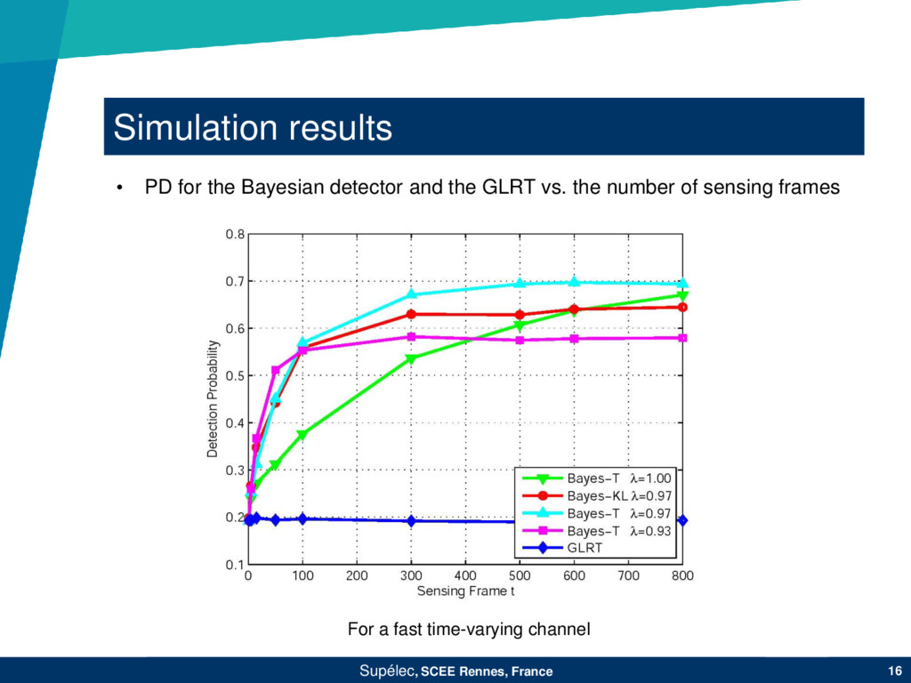
scheme also shows a better performance over one-shot detectors. A coarse approximation (thresholding-based approach) attain a better performance. In this case, a small degradation in its performance is observed by setting a higher value for λ =1.0. • A Bayesian detector show the feasibility of learning efficiently the posteriors parameters to detect a PU signal under stationary and non-stationary environments.
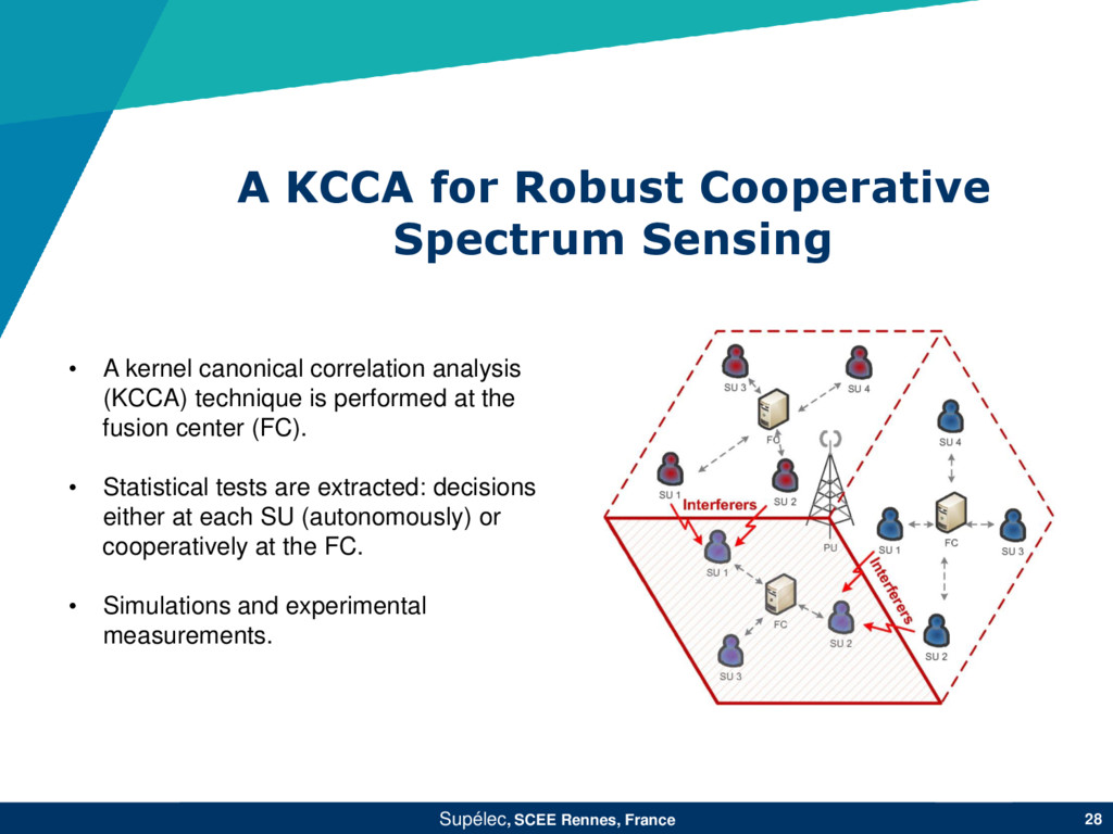
France 28 • A kernel canonical correlation analysis (KCCA) technique is performed at the fusion center (FC). • Statistical tests are extracted: decisions either at each SU (autonomously) or cooperatively at the FC. • Simulations and experimental measurements.
• The optimal detectors at each SU will be highly correlated, i.e. if SUs are either all under the null hypothesis or all under the alternative hypothesis. • The proposal aims to find the non-linear transformations of the measurements that provides maximal correlation. These non-linear transformations are employed to decide if the measurements come from the distribution p(r|1) or from p(r|0). • We consider M secondary users and a PU in the same area; and the signal model takes into account the presence of local interferences
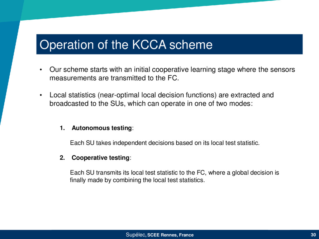
1. Autonomous testing: Each SU takes independent decisions based on its local test statistic. 2. Cooperative testing: Each SU transmits its local test statistic to the FC, where a global decision is finally made by combining the local test statistics. • Our scheme starts with an initial cooperative learning stage where the sensors measurements are transmitted to the FC. • Local statistics (near-optimal local decision functions) are extracted and broadcasted to the SUs, which can operate in one of two modes:
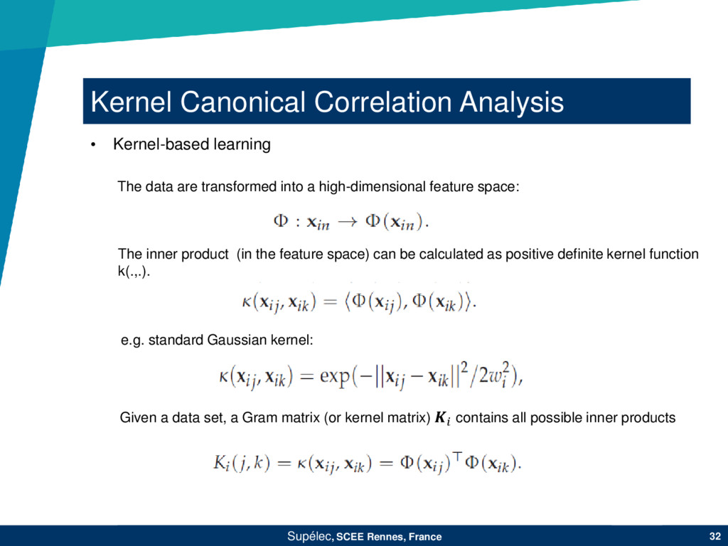
Kernel-based learning The data are transformed into a high-dimensional feature space: Given a data set, a Gram matrix (or kernel matrix) contains all possible inner products e.g. standard Gaussian kernel: The inner product (in the feature space) can be calculated as positive definite kernel function k(.,.).
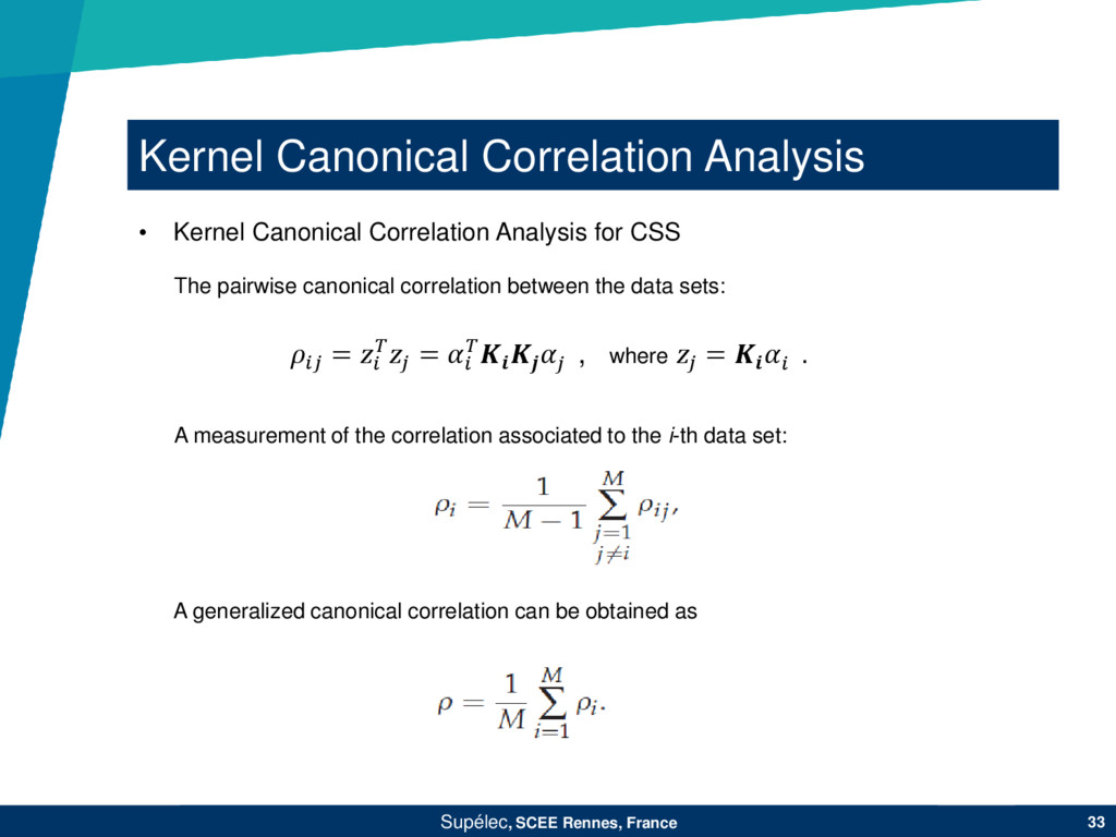
Kernel Canonical Correlation Analysis for CSS The pairwise canonical correlation between the data sets: A measurement of the correlation associated to the i-th data set: A generalized canonical correlation can be obtained as = = , where = .
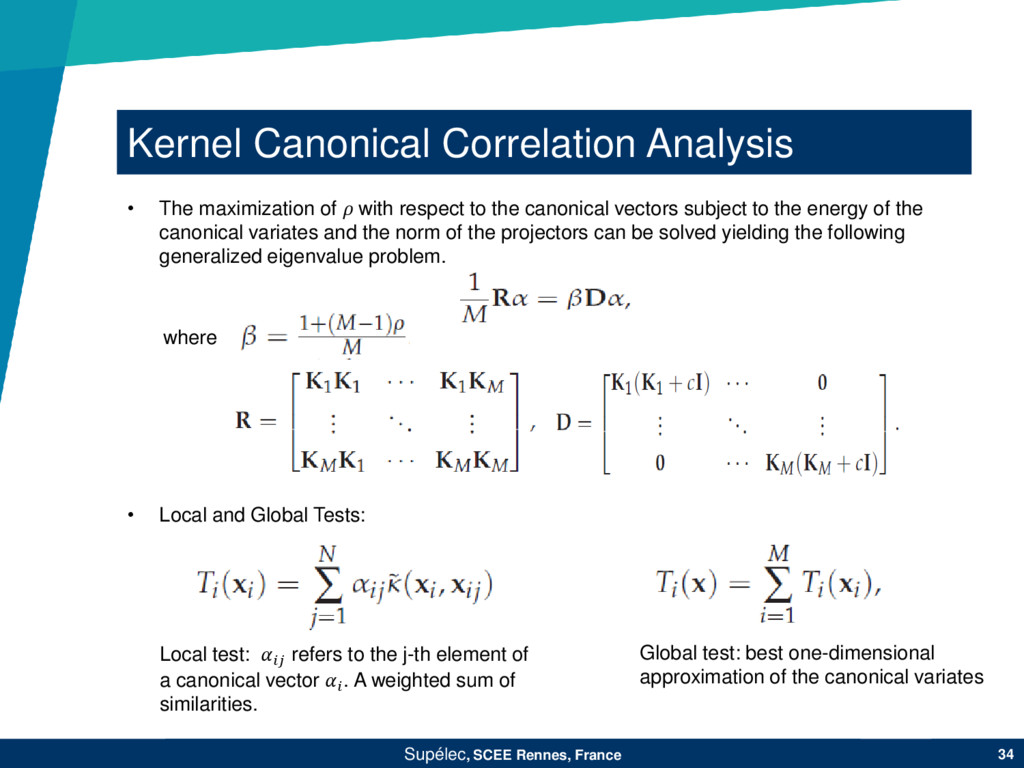
Local and Global Tests: Local test: refers to the j-th element of a canonical vector . A weighted sum of similarities. Global test: best one-dimensional approximation of the canonical variates • The maximization of with respect to the canonical vectors subject to the energy of the canonical variates and the norm of the projectors can be solved yielding the following generalized eigenvalue problem. where
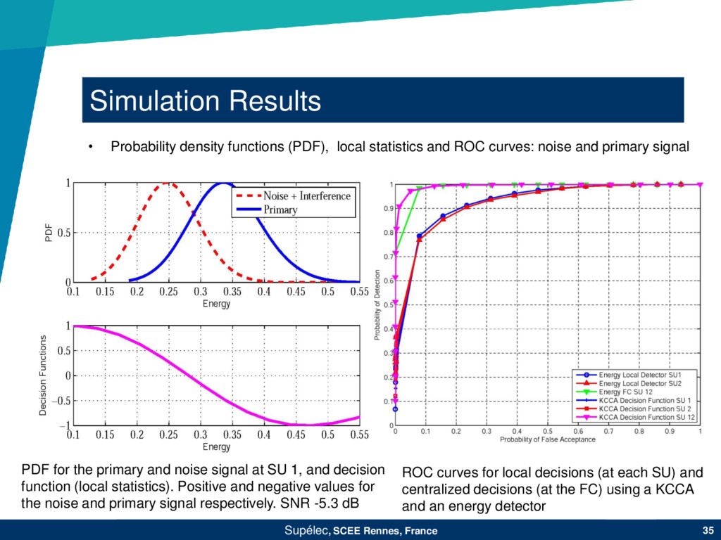
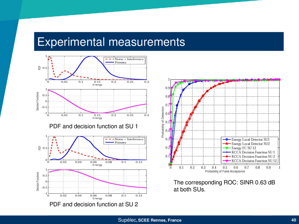
primary and noise signal at SU 1, and decision function (local statistics). Positive and negative values for the noise and primary signal respectively. SNR -5.3 dB ROC curves for local decisions (at each SU) and centralized decisions (at the FC) using a KCCA and an energy detector • Probability density functions (PDF), local statistics and ROC curves: noise and primary signal
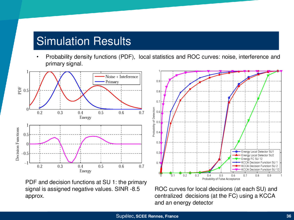
functions at SU 1: the primary signal is assigned negative values. SINR -8.5 approx. ROC curves for local decisions (at each SU) and centralized decisions (at the FC) using a KCCA and an energy detector • Probability density functions (PDF), local statistics and ROC curves: noise, interference and primary signal.
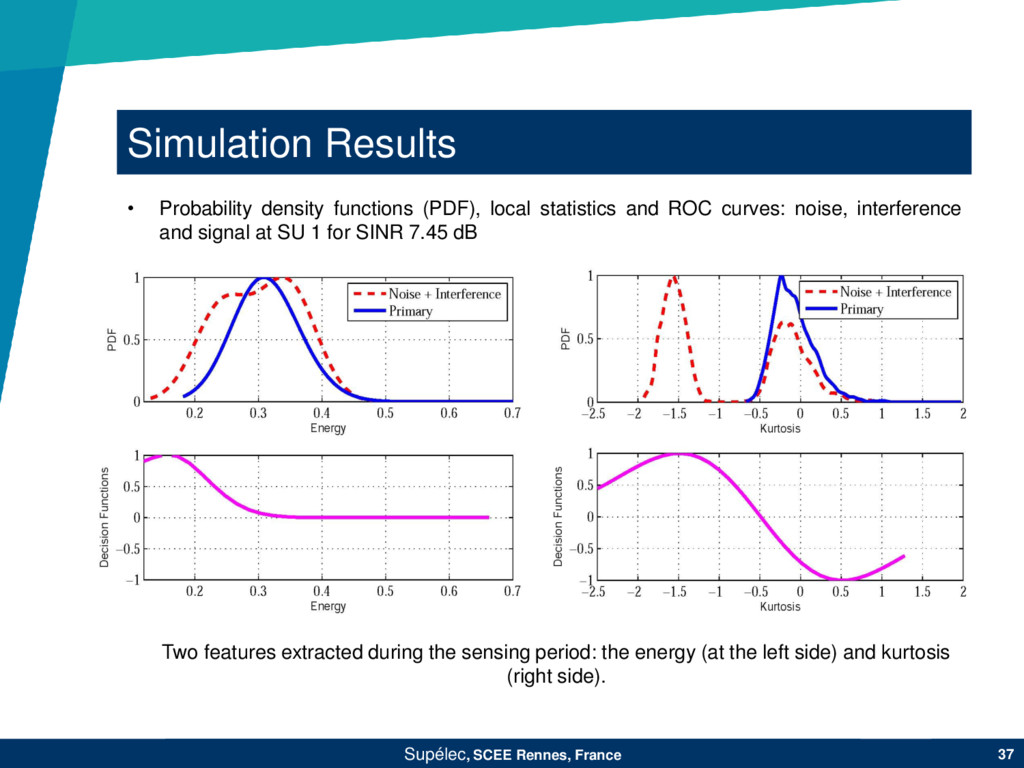
functions (PDF), local statistics and ROC curves: noise, interference and signal at SU 1 for SINR 7.45 dB Two features extracted during the sensing period: the energy (at the left side) and kurtosis (right side).
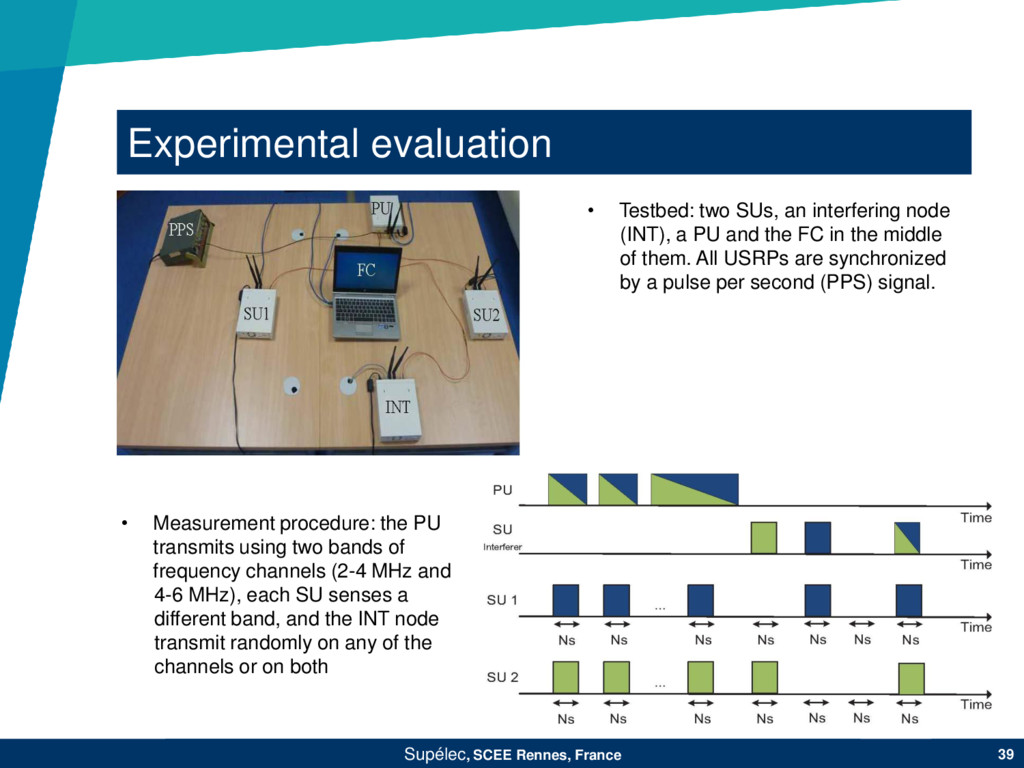
SUs, an interfering node (INT), a PU and the FC in the middle of them. All USRPs are synchronized by a pulse per second (PPS) signal. • Measurement procedure: the PU transmits using two bands of frequency channels (2-4 MHz and 4-6 MHz), each SU senses a different band, and the INT node transmit randomly on any of the channels or on both
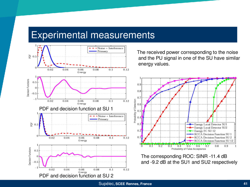
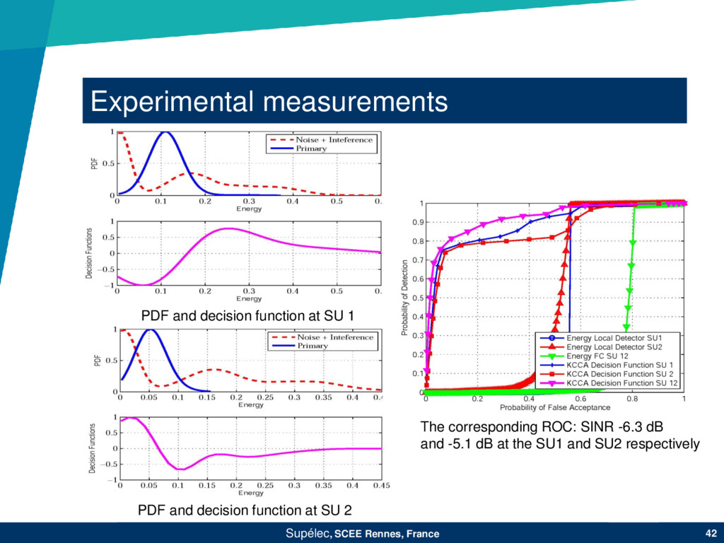
corresponding to the noise and the PU signal in one of the SU have similar energy values. PDF and decision function at SU 1 PDF and decision function at SU 2 The corresponding ROC: SINR -11.4 dB and -9.2 dB at the SU1 and SU2 respectively
has been evaluated under different scenarios in which noise or noise plus interference are present, and for which different features are extracted during the sensing period. • Our approach operates in blind manner, and can be applied to time-changing environments, since it adapts itself by retraining from time to time. • For scenarios with only noise and using only energy measurements: the KCCA and the energy detector attain the same performance, since the obtained tests are close to the optimal NP detector. • In scenarios with noise plus interference, our KCCA detector obtains a significant gain over an energy detector.
measurements: we corroborate the learning ability to detect the PU signal by exploiting the correlation among the received signals. • In fact, more challenging cases not taken into account in our simulation environment are also addressed, e.g. different noise variance at each SU as well as the interference power received at each SUs. • Our technique exhibits a much better performance than that of the energy detector as the interference level increases, since our KCCA framework exploits better the correlation of the received PU signal when more uncorrelated external interference is present.