Spatial Active Noise Control Based on Sound Field Interpolation Incorporating Physical Constraints

Keynote speech at IN-NOVA Days 2026

Transcript

1. Spatial Active Noise Control Based on Sound Field Interpolation Incorporating Physical Constraints Shoichi Koyama National Institute of Informatics, Japan
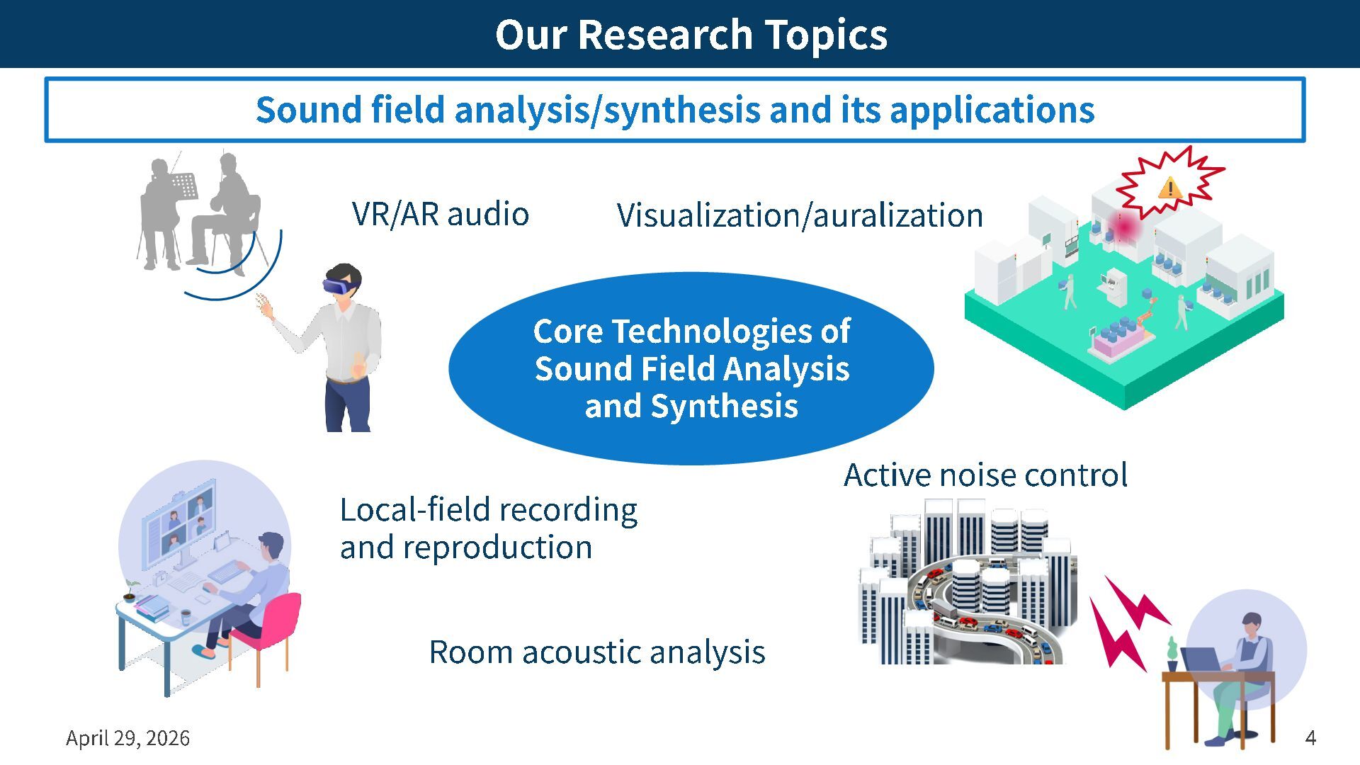
2. April 29, 2026 4 VR/AR audio Active noise control Local -field recording and reproduction Visualization/auralization Room acoustic analysis Our Research Topics Sound field analysis/synthesis and its applications Core Technologies of Sound Field Analysis and Synthesis
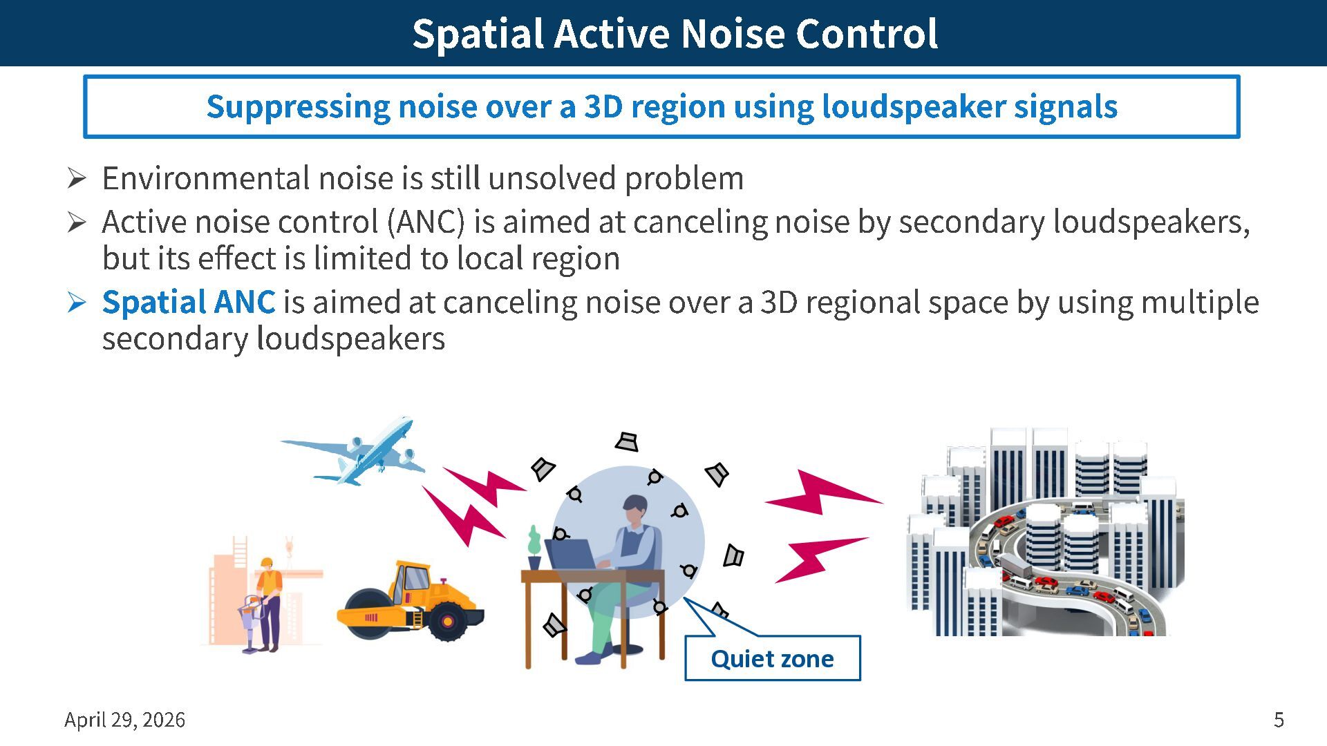
3. Spatial Active Noise Control ➢ Environmental noise is still unsolved problem ➢ Active noise control (ANC) is aimed at canceling noise by secondary loudspeakers, but its effect is limited to local region ➢ Spatial ANC is aimed at canceling noise over a 3D regional space by using multiple secondary loudspeakers April 29, 2026 5 Suppressing noise over a 3D region using loudspeaker signals Quiet zone
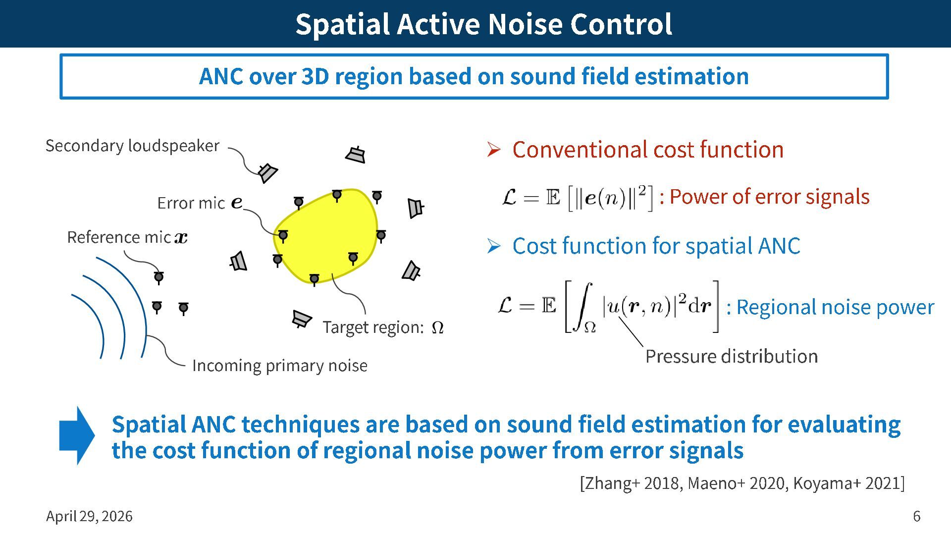
4. Spatial Active Noise Control April 29, 2026 6 ANC over 3D region based on sound field estimation ➢ Conventional cost function ➢ Cost function for spatial ANC : Power of error signals : Regional noise power Error mic Secondary loudspeaker Incoming primary noise Reference mic Target region: Spatial ANC techniques are based on sound field estimation for evaluating the cost function of regional noise power from error signals [Zhang+ 2018, Maeno+ 2020, Koyama+ 2021] Pressure distribution
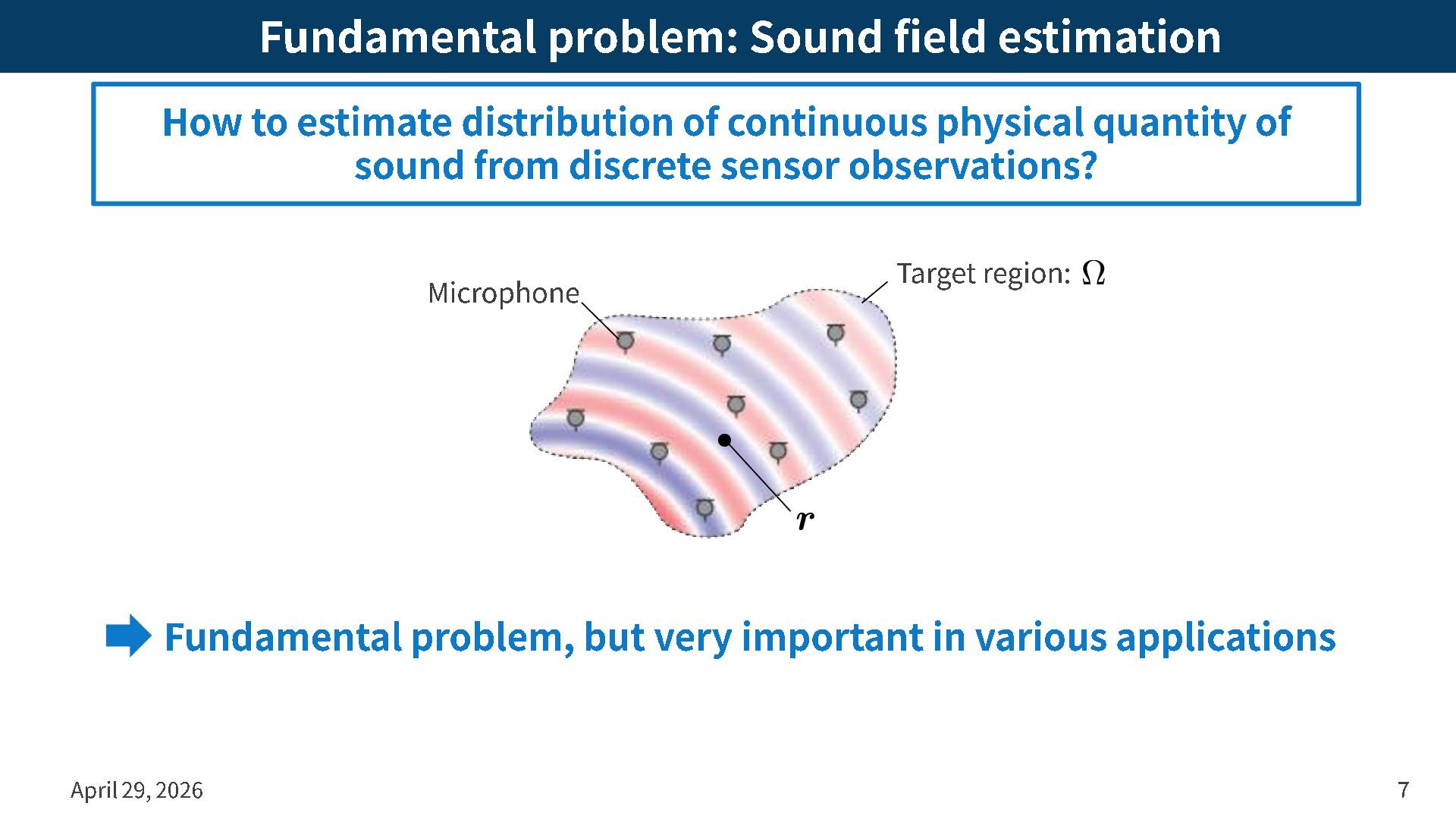
5. Fundamental problem: Sound field estimation April 29, 2026 7 How to estimate distribution of continuous physical quantity of sound from discrete sensor observations? Target region: Microphone Fundamental problem, but very important in various applications
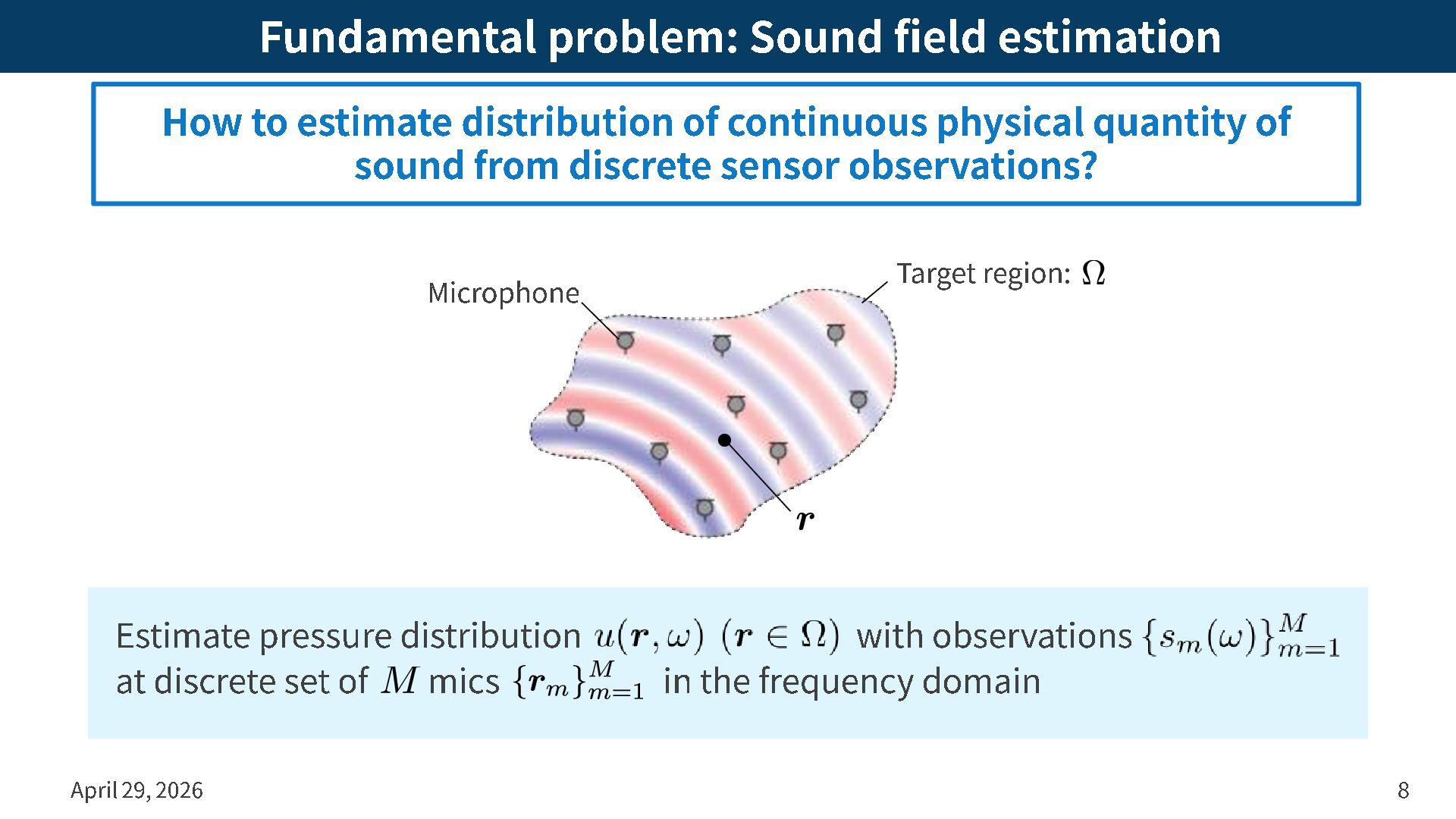
6. Fundamental problem: Sound field estimation April 29, 2026 8 How to estimate distribution of continuous physical quantity of sound from discrete sensor observations? Estimate pressure distribution with observations at discrete set of mics in the frequency domain Target region: Microphone
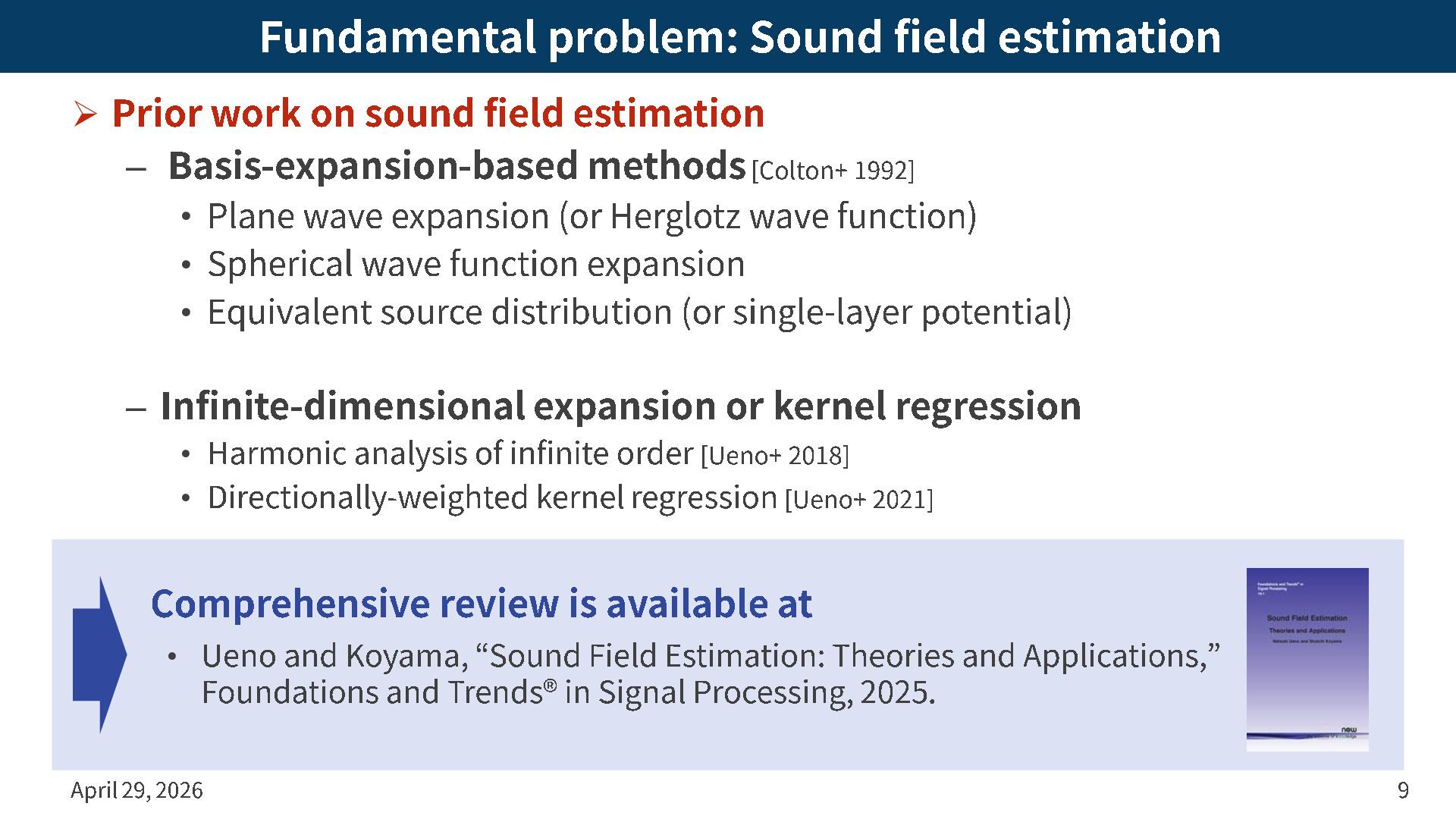
7. Fundamental problem: Sound field estimation ➢ Prior work on sound field estimation – Basis -expansion -based methods [Colton+ 1992] • Plane wave expansion (or Herglotz wave function) • Spherical wave function expansion • Equivalent source distribution (or single -layer potential) – Infinite -dimensional expansion or kernel regression • Harmonic analysis of infinite order [Ueno+ 2018] • Directionally -weighted kernel regression [Ueno+ 2021] April 29, 2026 9 Comprehensive review is available at • Ueno and Koyama, “Sound Field Estimation: Theories and Applications, ” Foundations and Trends ®️ in Signal Processing, 2025 .
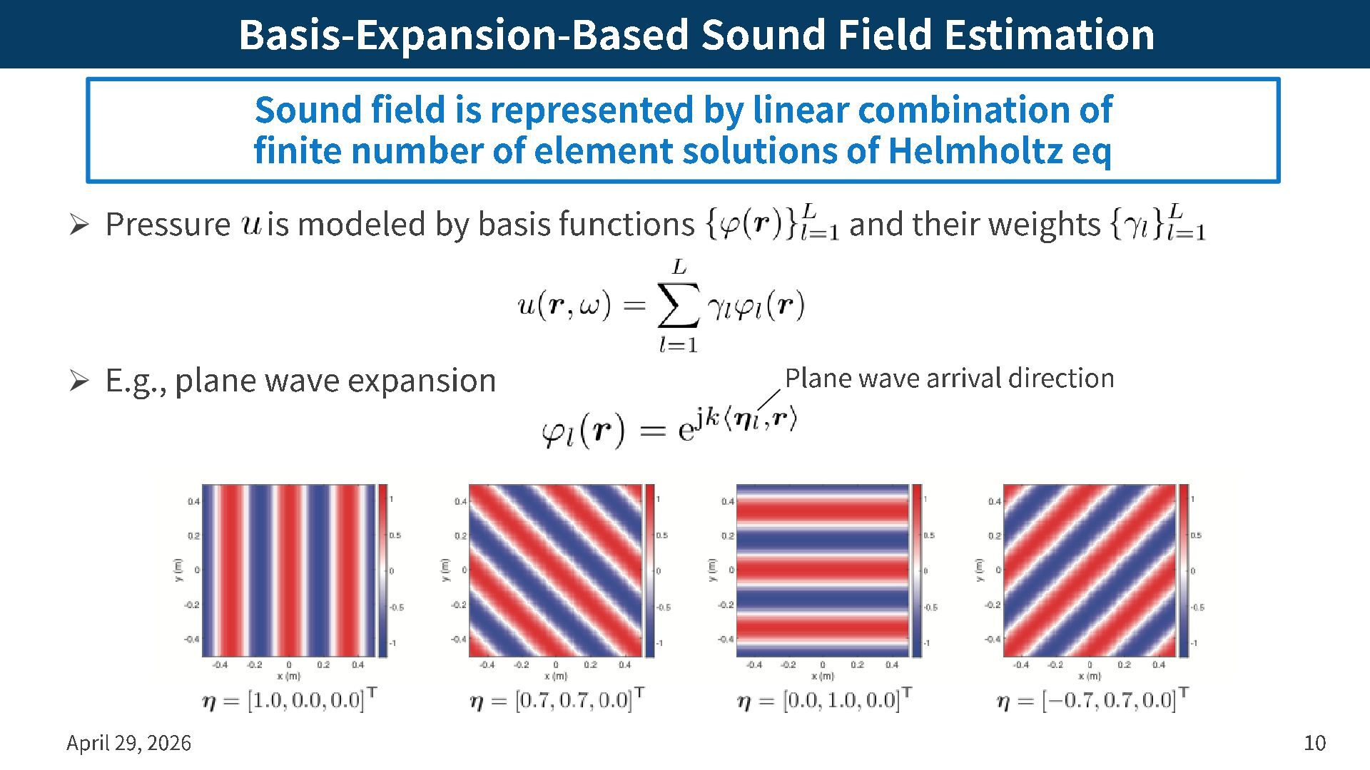
8. Basis -Expansion -Based Sound Field Estimation ➢ Pressure is modeled by basis functions and their weights ➢ E.g., plane wave expansion April 29, 2026 10 Sound field is represented by linear combination of finite number of element solutions of Helmholtz eq Plane wave arrival direction
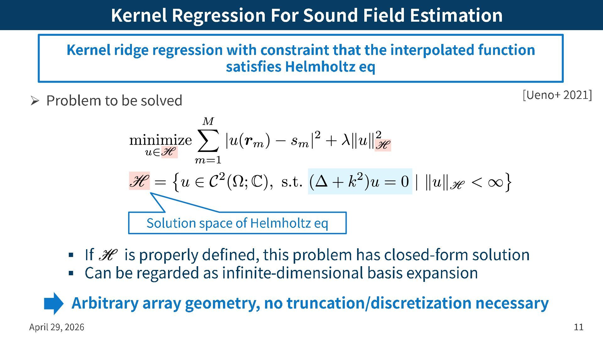
9. Kernel Regression For Sound Field Estimation ➢ Problem to be solved April 29, 2026 11 Kernel ridge regression with constraint that the interpolated function satisfies Helmholtz eq [Ueno+ 2021] Arbitrary array geometry, no truncation/discretization necessary ▪ If is properly defined, this problem has closed -form solution ▪ Can be regarded as infinite -dimensional basis expansion Solution space of Helmholtz eq
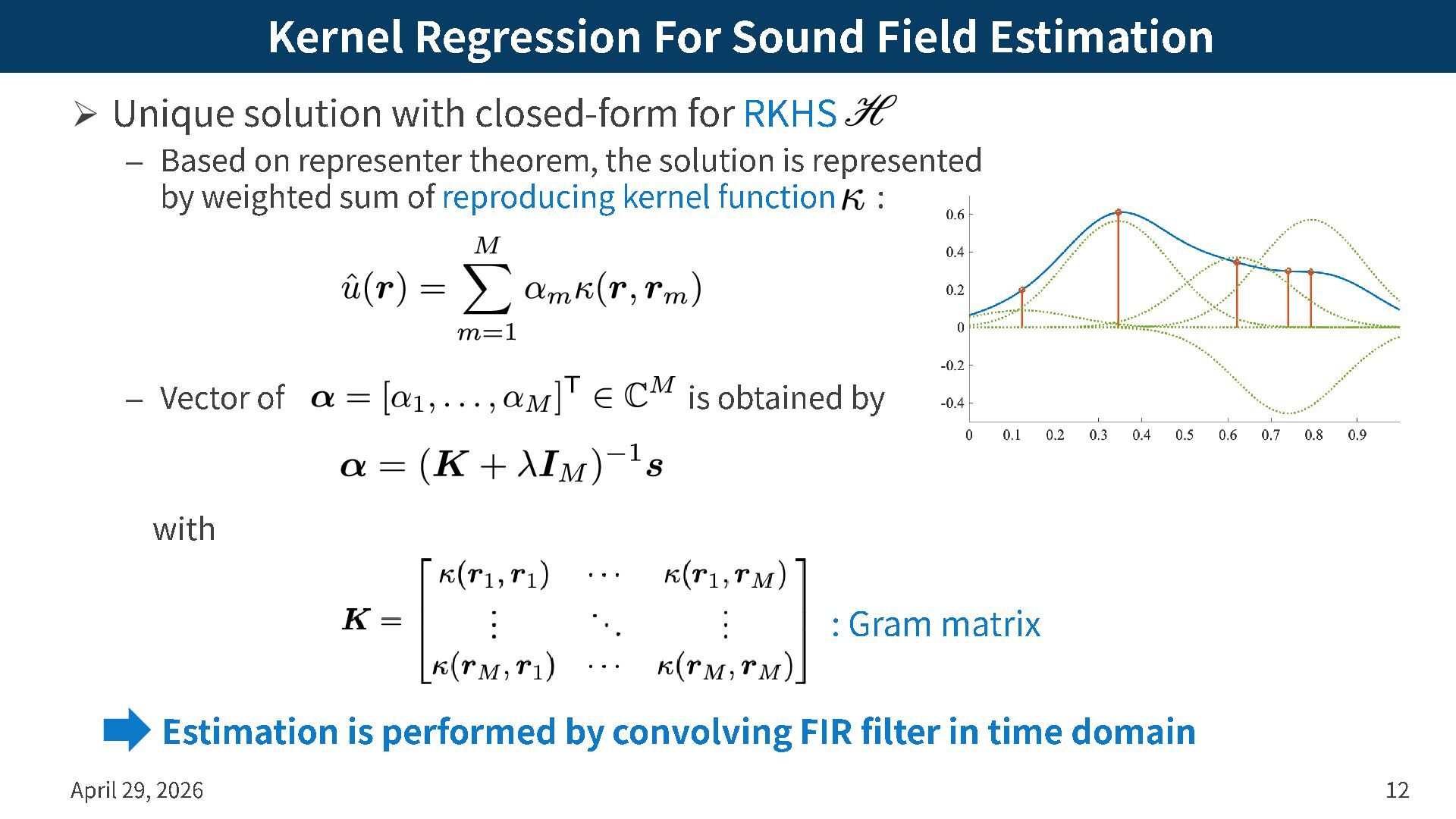
10. Kernel Regression For Sound Field Estimation ➢ Unique solution with closed -form for RKHS – Based on representer theorem , the solution is represented by weighted sum of reproducing kernel function : – Vector of is obtained by with April 29, 2026 12 Estimation is performed by convolving FIR filter in time domain : Gram matrix
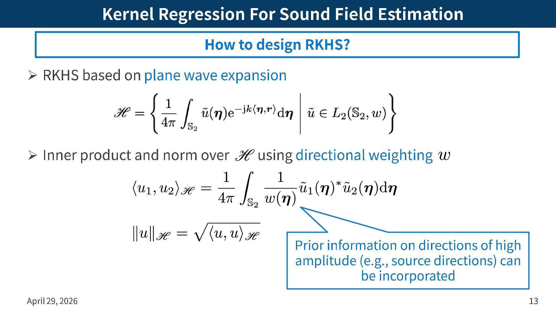
11. Kernel Regression For Sound Field Estimation ➢ RKHS based on plane wave expansion ➢ Inner product and norm over using directional weighting April 29, 2026 13 How to design RKHS? Prior information on directions of high amplitude (e.g., source directions) can be incorporated
12. Kernel Regression For Sound Field Estimation ➢ Kernel function for based on von Mises –Fisher distribution ➢ When no prior information, i.e., uniform weight , April 29, 2026 14 How to design RKHS? with
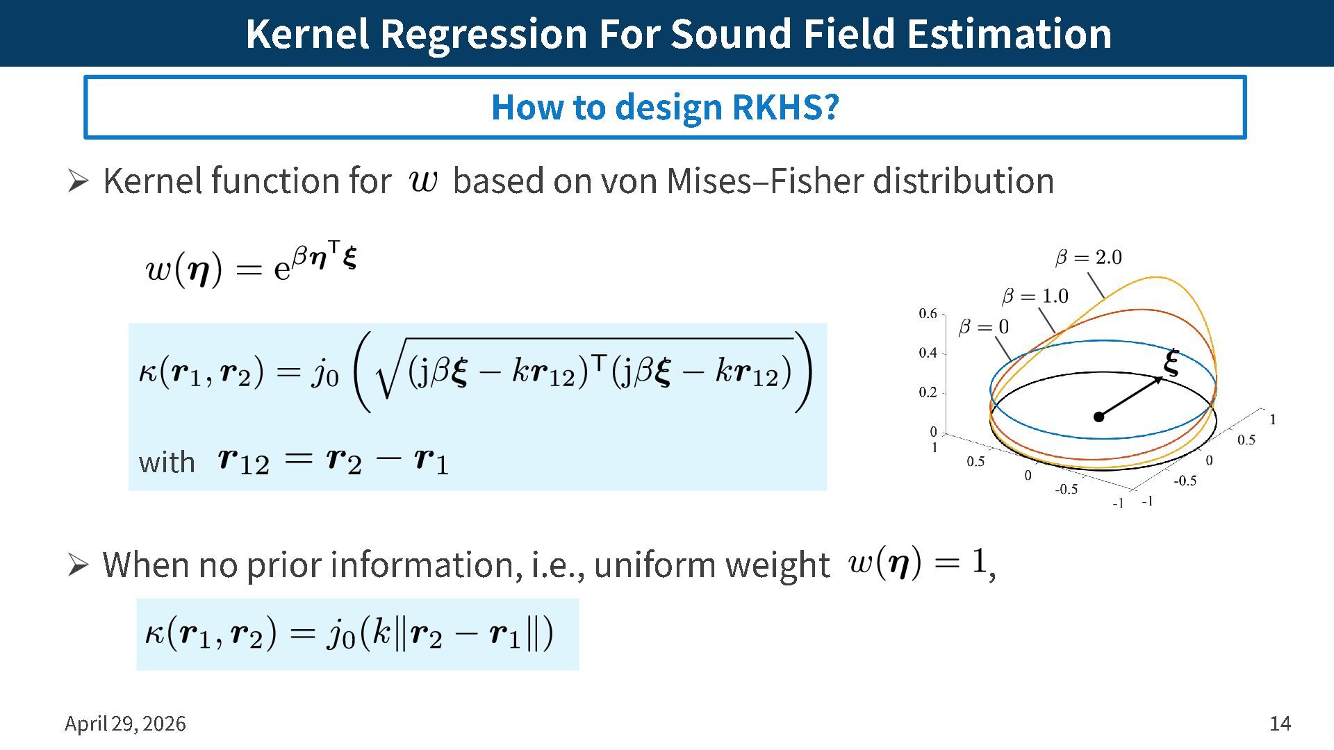
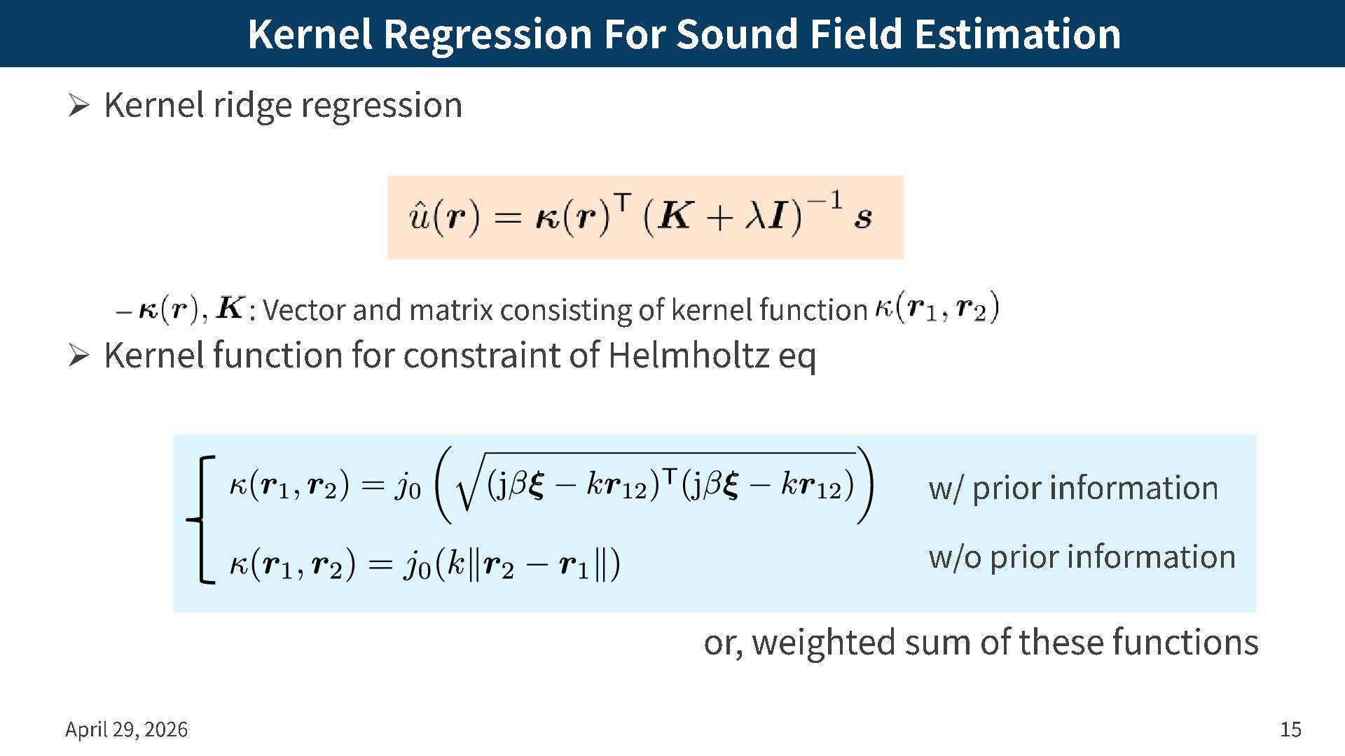
13. Kernel Regression For Sound Field Estimation ➢ Kernel ridge regression – : Vector and matrix consisting of kernel function ➢ Kernel function for constraint of Helmholtz eq April 29, 2026 15 w/ prior information w/o prior information or, weighted sum of these functions
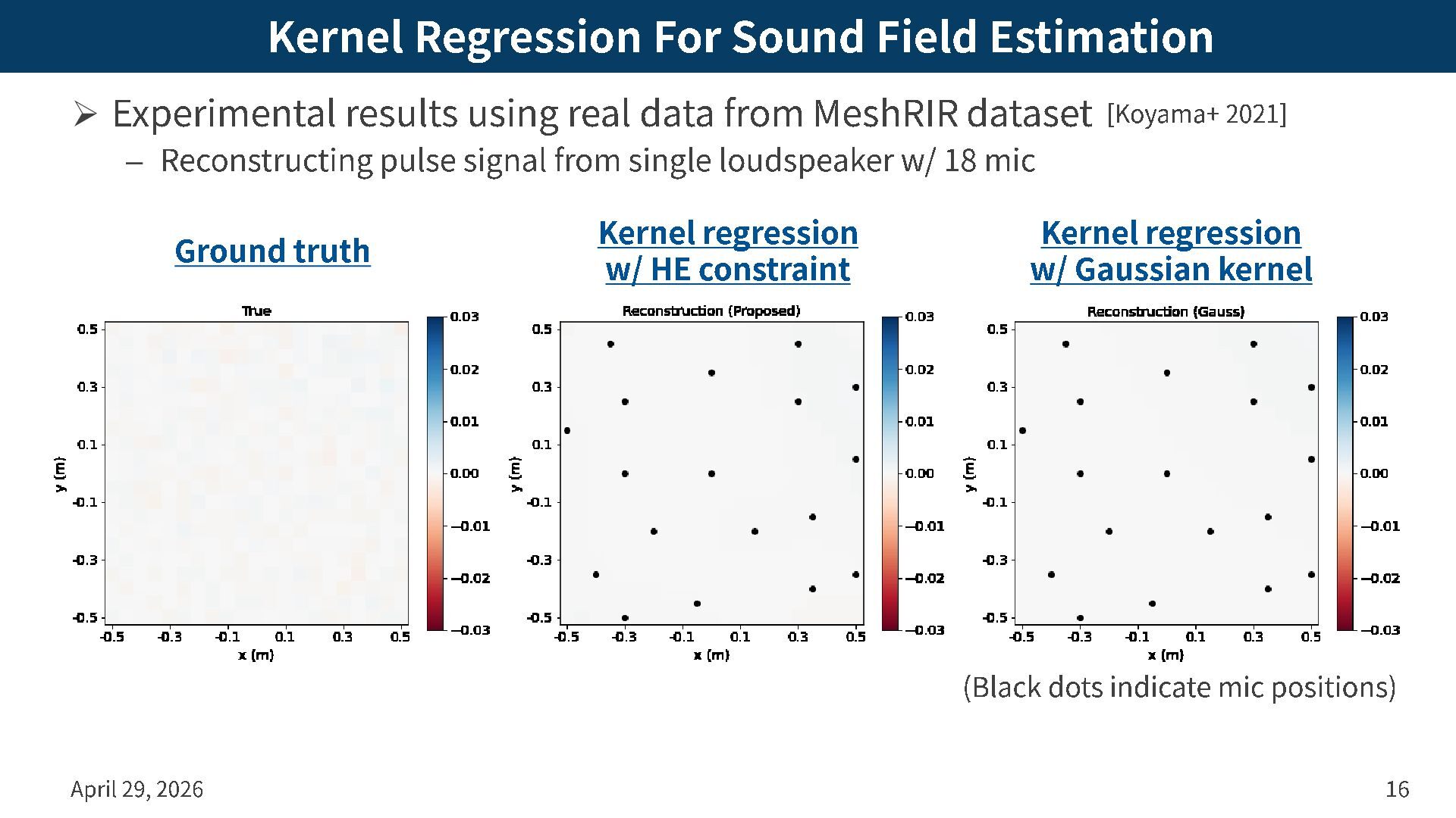
14. Kernel Regression For Sound Field Estimation ➢ Experimental results using real data from MeshRIR dataset – Reconstructing pulse signal from single loudspeaker w/ 18 mic April 29, 2026 16 Ground truth Kernel regression w/ HE constraint Kernel regression w/ Gaussian kernel (Black dots indicate mic positions) [Koyama+ 2021]
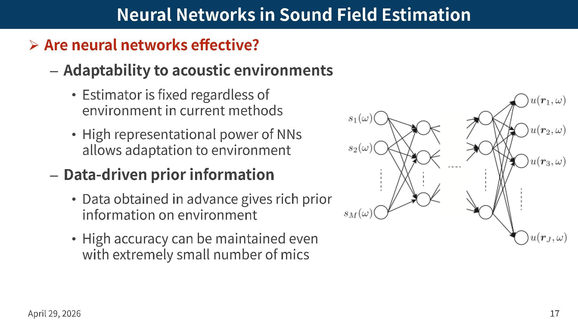
15. Neural Networks in Sound Field Estimation ➢ Are neural networks effective? – Adaptability to acoustic environments • Estimator is fixed regardless of environment in current methods • High representational power of NNs allows adaptation to environment – Data -driven prior information • Data obtained in advance gives rich prior information on environment • High accuracy can be maintained even with extremely small number of mics April 29, 2026 17
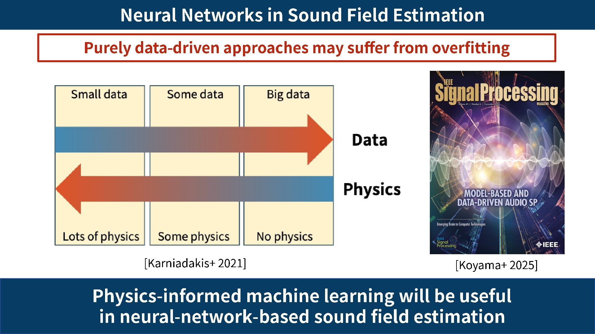
16. Neural Networks in Sound Field Estimation April 29, 2026 18 Purely data -driven approaches may suffer from overfitting [Karniadakis+ 2021] [Koyama+ 2025] Physics -informed machine learning will be useful in neural -network -based sound field estimation
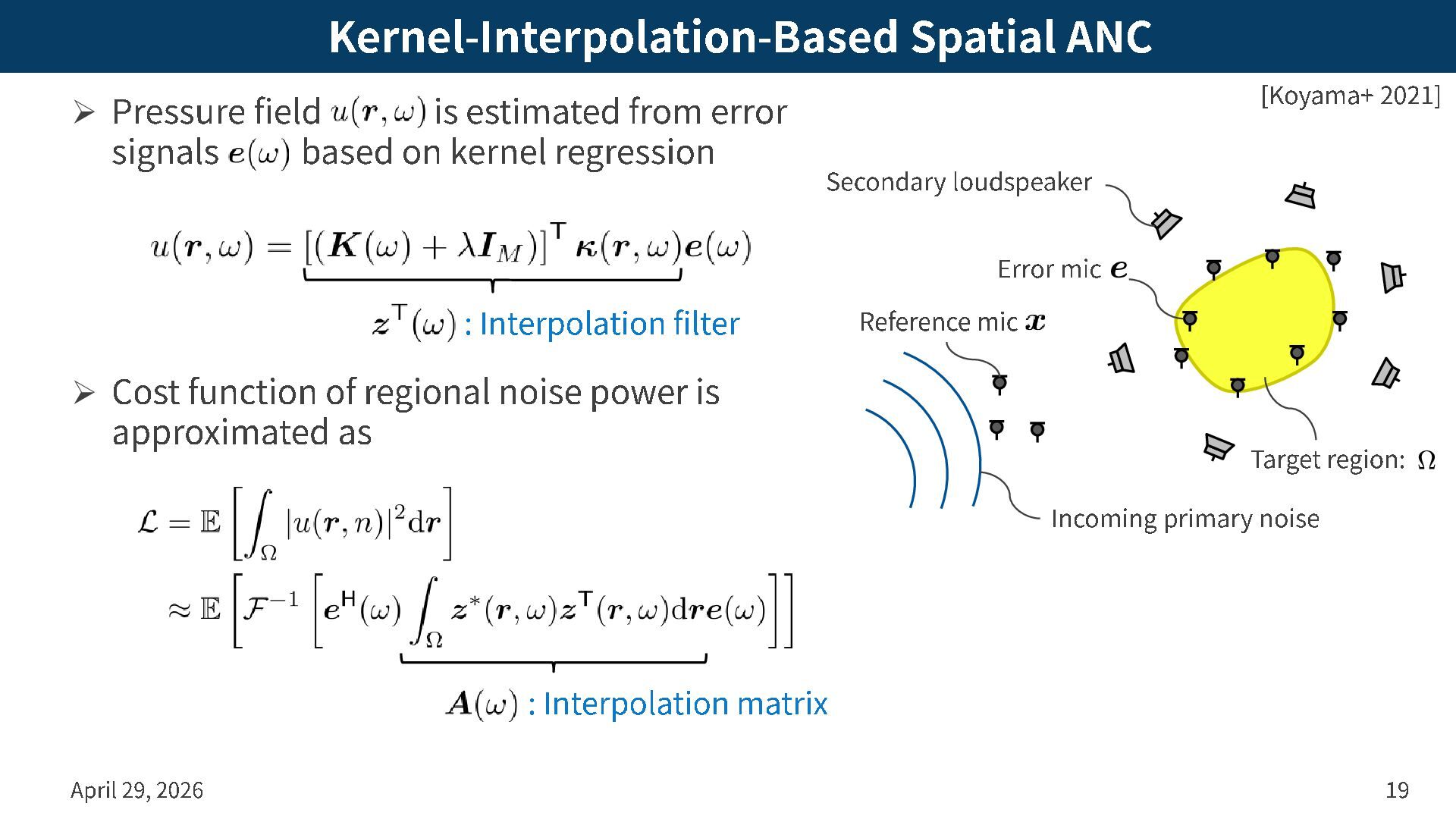
17. Kernel -Interpolation -Based Spatial ANC ➢ Pressure field is estimated from error signals based on kernel regression ➢ Cost function of regional noise power is approximated as April 29, 2026 19 : Interpolation filter : Interpolation matrix [Koyama+ 2021] Error mic Secondary loudspeaker Incoming primary noise Reference mic Target region:
18. Kernel -Interpolation -Based Spatial ANC ➢ Gradient of the cost function w.r.t. filter matrix ➢ Kernel -interpolation -based FxLMS algorithm April 29, 2026 20 Error mic Secondary loudspeaker Incoming primary noise Reference mic Target region: Secondary path Truncated and delayed interpolation matrix [Koyama+ 2021]
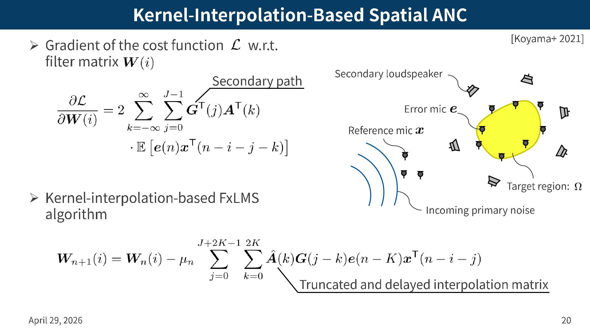
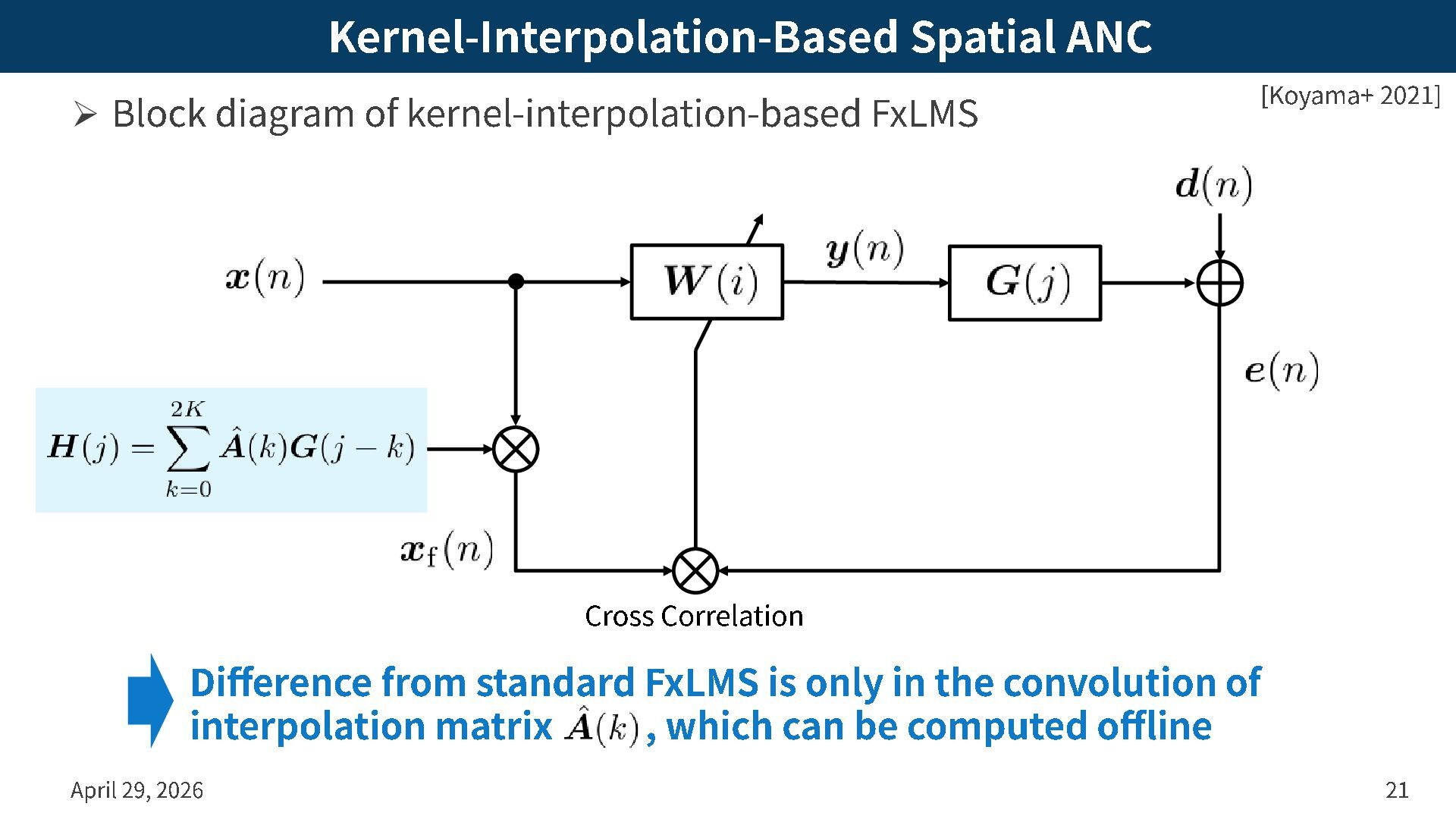
19. Kernel -Interpolation -Based Spatial ANC ➢ Block diagram of kernel -interpolation -based FxLMS April 29, 2026 21 [Koyama+ 2021] Difference from standard FxLMS is only in the convolution of interpolation matrix , which can be computed offline Cross Correlation
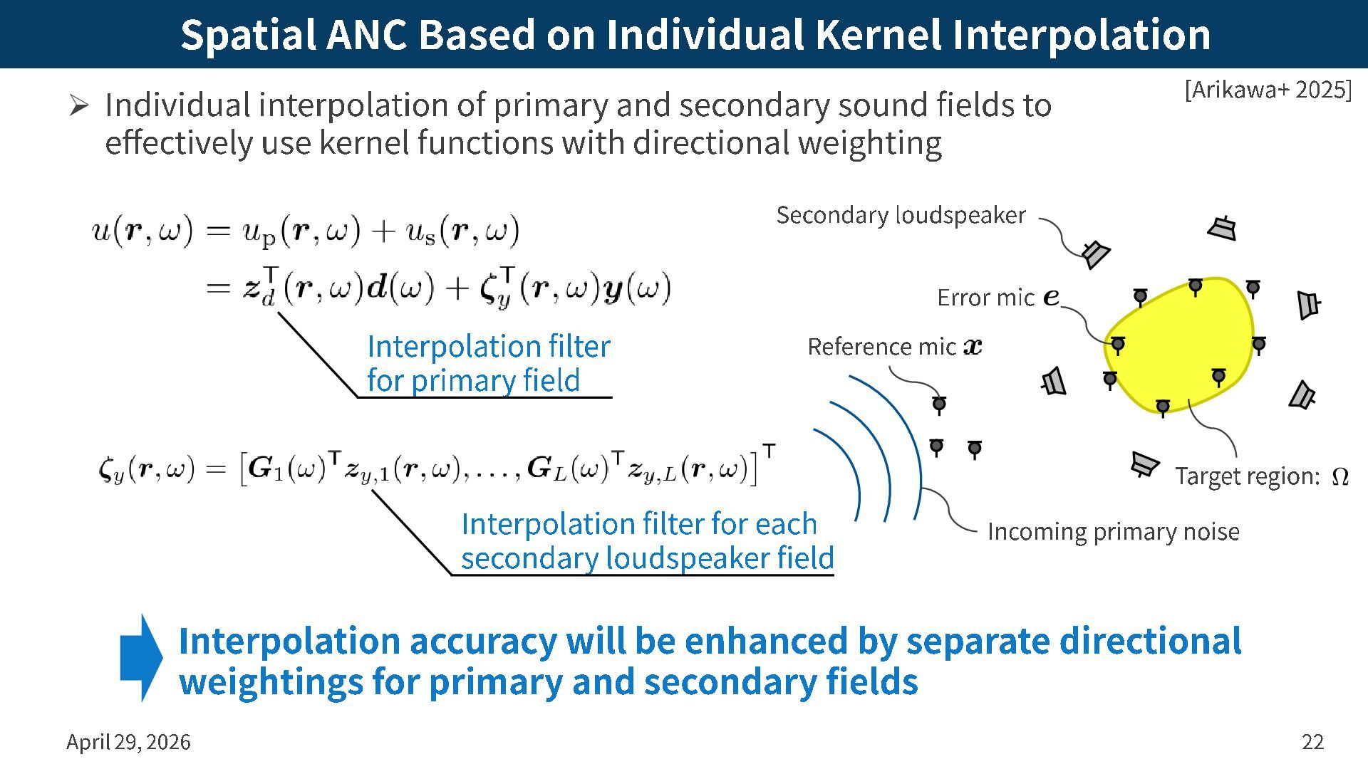
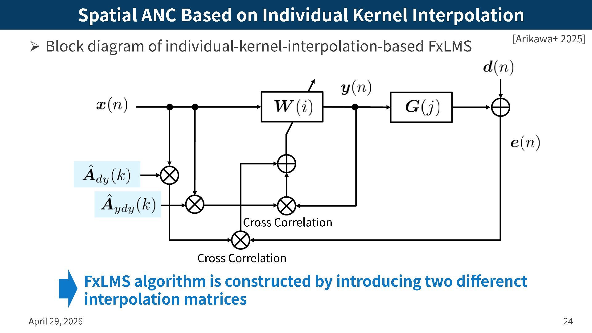
20. Spatial ANC Based on Individual Kernel Interpolation ➢ Individual interpolation of primary and secondary sound fields to effectively use kernel functions with directional weighting April 29, 2026 22 [Arikawa+ 2025 ] Error mic Secondary loudspeaker Incoming primary noise Reference mic Target region: Interpolation accuracy will be enhanced by separate directional weightings for primary and secondary fields Interpolation filter for primary field Interpolation filter for each secondary loudspeaker field
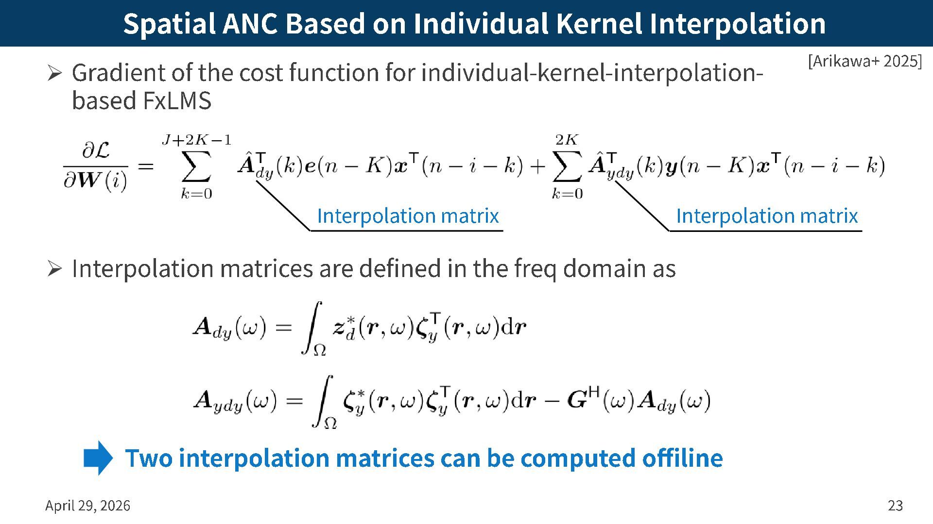
21. Spatial ANC Based on Individual Kernel Interpolation ➢ Gradient of the cost function for individual -kernel -interpolation - based FxLMS ➢ Interpolation matrices are defined in the freq domain as April 29, 2026 23 [Arikawa+ 2025 ] Interpolation matrix Interpolation matrix Two interpolation matrices can be computed offiline
22. Spatial ANC Based on Individual Kernel Interpolation ➢ Block diagram of individual -kernel -interpolation -based FxLMS April 29, 2026 24 FxLMS algorithm is constructed by introducing two differenct interpolation matrices [Arikawa+ 2025 ] Cross Correlation Cross Correlation
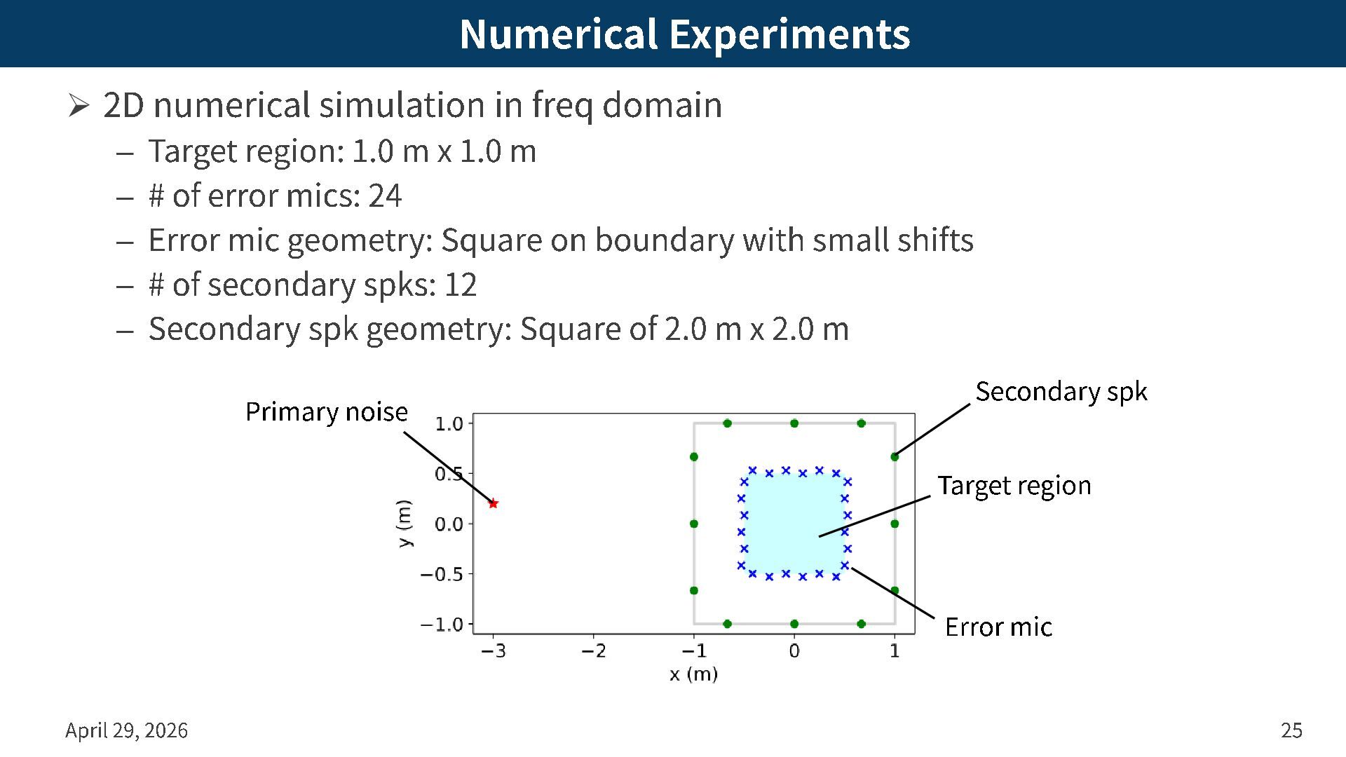
23. Numerical Experiments ➢ 2D numerical simulation in freq domain – Target region: 1.0 m x 1.0 m – # of error mics: 24 – Error mic geometry: Square on boundary with small shifts – # of secondary spks: 12 – Secondary spk geometry: Square of 2.0 m x 2.0 m April 29, 2026 25 Primary noise Secondary spk Error mic Target region
24. Numerical Experiments ➢ Pressure and normalized power distributions at 700 Hz April 29, 2026 26 KI -FxLMS FxLMS Pressure Power
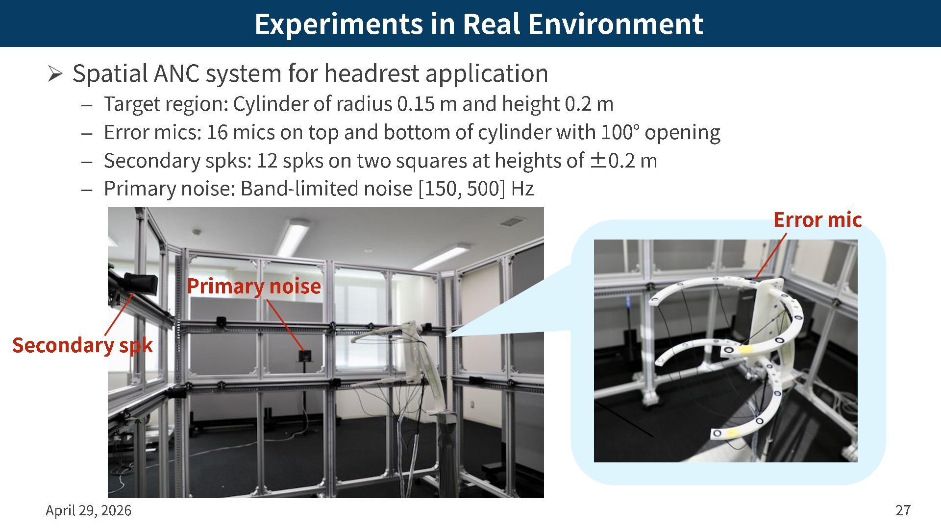
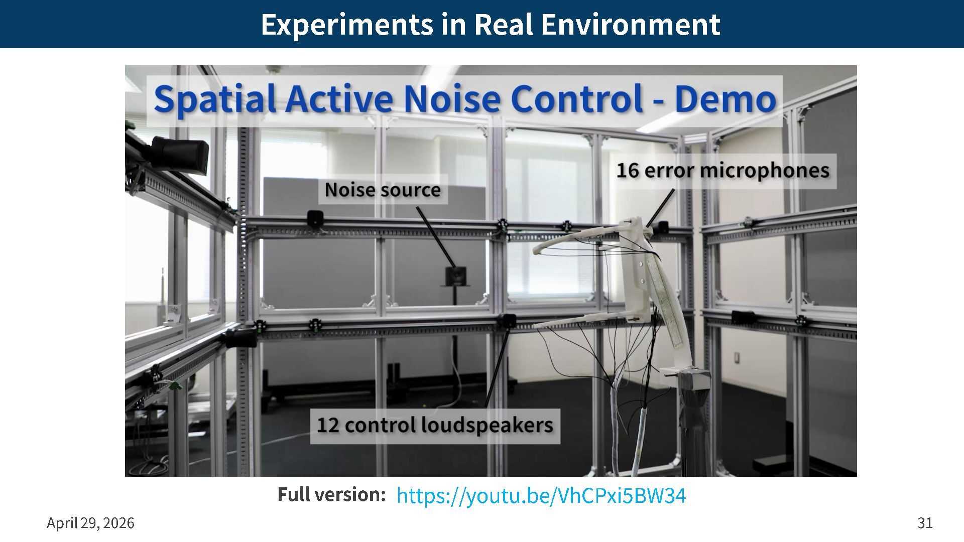
25. Experiments in Real Environment ➢ Spatial ANC system for headrest application – Target region: Cylinder of radius 0.15 m and height 0.2 m – Error mics: 16 mics on top and bottom of cylinder with 100 ° opening – Secondary spks: 12 spks on two squares at heights of ± 0.2 m – Primary noise: Band -limited noise [150, 500] Hz April 29, 2026 27 Primary noise Secondary spk Error mic
26. Experiments in Real Environment ➢ Filter convergence in offline adaptation April 29, 2026 28
27. Experiments in Real Environment ➢ Noise reduction at 12 evaluation points inside the target area April 29, 2026 29 FxLMS KI -FxLMS (Total) KI -FxLMS (Individual)
28. Experiments in Real Environment ➢ Power spectrum comparison at evaluation point #2 April 29, 2026 30
29. Experiments in Real Environment April 29, 2026 31 https:// youtu.be /VhCPxi5BW34 Full version:
30. Conclusion ➢ Spatial ANC based on kernel interpolation of sound fields – Fundamental problem in spatial ANC is sound field estimation – Kernel regression with constraint of Helmholtz eq allows estimating continuous sound field from discrete mics by linear operation – Cost function defined as regional noise power within the target region can be approximated by error signals via kernel regression – FxLMS algorithm for kernel -interpolation -based spatial ANC is achieved by introducing additional interpolation matrix – Numerical and practical experiments indicated spatial ANC techniques can adequately suppress noise within a 3D target region April 29, 2026 32 Physics -informed machine learning will open up new applications for sound field analysis and control Thank you for your attention!